Pose Normalization based on Kernel ELM Regression for Face Recognition

Published Online May 2017 in MECS DOI: 10.5815/ijigsp.2017.05.07

Face recognition is used extensively for biometric identification since last two decades. The popularity of face recognition system is due to its advantages of being passive and non-intrusive nature. It also provides higher recognition accuracy as compared to other biometric identification techniques. However, it suffers from serious challenges under outdoor environments, for example, appearance of the face may vary too much due to different poses. In current reviews [1,2], pose variation is identified as one of the main unsolved problem for face recognition system. Therefore, it has attracted the interest of many researchers to normalize the pose variations.

A lot of approaches have been proposed to deal with recognizing faces under different poses. View based methods [3-8] were mainly used for pose normalization, but it usually requires multiple face images of each subject with different poses. 3D model based methods [920] are also explored to normalize the pose variations, but these methods are too slow to use them in real time scenario.

Generating virtual frontal view from its non frontal view [21-28] is one of the popular solution to normalize pose for face recognition. By generating the virtual frontal view of the posed image, either, all face images are normalized to the frontal view or gallery can be extended to cover the large pose variations.

Local linear regression (LLR) method is proposed by Chai et al. [24] for efficiently generating the virtual frontal view for the posed face image. In this method, the posed image is partitioned into multiple patches and then linear regression is applied to each patch for predicting its corresponding virtual frontal patch. LLR method to normalize pose variations is simpler as well as easier for real world tasks as only linear regression has to be done. Also, it requires only the coarse alignment based on the center of the two eyes. However, main drawback of linear assumption is the loss of lots of information, as the rotation of the human head is a non linear problem. Therefore, to deal with non linearity of rotation of human head, there is the need of non linear regression to solve the pose variations.

In this paper, kernel extreme learning machine (KELM) regression [31-34] is proposed to efficiently estimate the virtual frontal face image from its non frontal view. Kernel ELM is used here as the face image is non linear in shape and the different poses change non linearly. Linear regression cannot estimate these non linear changes accurately. Compared to linear regression, KELM regression is more efficient for virtual view generation as it considers non linear shape of the face view.

The remaining paper is organized as: Section 2 gives the review of existing techniques for pose normalization. Section 3 explains the linear regression for virtual view generation. Section 4 explains the KELM regression for generating the virtual frontal face view. Section 5 presents the results on GTAV face database. The conclusion and further recommendations for pose normalization is presented in Section 6.

• II.    Related Works

In literature, a much work has been done to normalize the pose variations [3-29] for efficient face recognition system. The pose normalization techniques are broadly categorized into three categories: (1) view based techniques, (2) 3D techniques, and (3) to generate virtual frontal face image techniques.

In view based techniques, [3-5] eigen faces are estimated from gallery input images to handle the pose problem. View based eigen space technique [3], at first determines the location and orientation of the target object by selecting the eigen vectors which best describes the image. The view based approach is further extended to the modular representation which provides robustness to the pose variations in the face image. The limitation of the view based technique is that it needs multiple posed images for each subject which is not often possible for real world applications. Eigen light fields (ELF) is presented by [6], in which the subject's head eigen light fields are calculated from the input gallery images and then matching between the input and test face image is done to recognize the faces. Eigen light field is obtained by eigen decomposing of light fields using principal component analysis (PCA) [7]. Light fields indicates the radiance of light in the free space [8]. The advantage of ELF is that only training set requires multiple posed image for each subject which can be possible. The limitation of ELF is its precise calculations for computing light fields.

3D model is one of the successful approach for pose normalization. The reason of success of 3D model based approaches for pose normalization is that the human heads are 3D objects and any changes in pose take place in 3D spaces. The 3D models can be reconstructed from their 2D face images using the techniques given in [9-14]. Martin and Rajwade [15] gives two-step normalization strategy for generating frontal posed image. In first step, support vector regression is used for coarse normalization which is followed by improve version of Iterated Closest Algorithm (ICA) to improve the pose alignment. Asthana et al. [16] proposed 3D pose normalization method in which first robust method is used to find the facial landmark points. These points are used to normalize the angle of the face and then the regression function is used to estimate the pitch and yaw angles. The estimated pose angle and landmark points are used to align 3D head model. Ding et al. [17] presents automatic continuous pose normalization based on improved multiview random forest embedded-active shape model (RFE-ASM) feature detector. Marsico et al. [18] presents the novel framework for pose and illumination normalization, named Face Analysis for Commercial Entities (FACE). Wang et al. [19] presents pose normalization via robust 3D shape reconstruction. 2D to 3D landmark correspondence for each 2D face image is learned by iteratively refining the 3D landmarks and their weighing coefficients. Zhu et al. [20] uses 3D Morphable Model to generate the frontal pose image. The results obtained using 3D models show best performance for pose normalization but it is highly computational procedure and also it is too slow to be used in real world applications.

Virtual frontal view generation techniques generally estimate the virtual view from its posed view directly in 2D domain. Vetter et. al . [21, 22] proposed linear object class which is applied separately into the shape vector and texture vector of the face image. Then the virtual images are obtained by combining the regenerated shape and texture vector by using the basis set of 2D prototypes. Chai et al. proposed [23] affine transformation to normalize the input pose image into the frontal face view. In this approach, face region is divided into three rectangles and then affine transformation is used to align the input posed face image to virtual frontal view. The main drawback of this approach is that it can normalize pose variations up to 30⁰ face rotation angle. Further, face rotation is non linear transformation, therefore, only affine transform cannot model the pose variations completely. Local linear regression (LLR) [24-25] efficiently generates virtual frontal face image from its corresponding non frontal view by estimating the pixel wise correspondence between the face images. In this technique, face image is partitioned into multiple local patches and then linear regression is applied to each non frontal patch to predict its corresponding frontal patch. Hsieh et. al. [26] proposed kernel based virtual frontal view generation method which integrates the non linearity of the kernel function and effectiveness of linear regression technique. This non linear mapping makes the results more accurate to the frontal view. Component wise pose normalization [27] for face recognition do the component wise pose normalization to generate the virtual frontal view. In this method, first the non frontal posed image is partitioned into different facial components and then virtual frontal view of each component is estimated by using LLR. Virtual frontal face is generated finally by integrating these virtual frontal components. Pose normalization using Markov Random Fields (MRF) [28] uses MRF to generate virtual frontal view from non frontal face image. Samet et al. [29] uses 2D PCA for feature extraction and then LLR to generate virtual frontal face image from different posed image.

• III.    Linear Regression for Virtual View Generation

For predicting the virtual frontal face from its non frontal view, Chai et. al. [24] devised this problem as the regression task. For explaining the linear regression for pose estimation, let {(7p°, ppk)} as the training set in which Ip° denotes the frontal training images set and Ipk denotes its corresponding posed image set. Here, Ip° = (Ip°,Ip°,..,Ip°) is the frontal image set and Ipk = (Ipk,Ipk,.,, p^)) is its corresponding posed image set. The non frontal face image Ipk is transformed into its corresponding frontal face view by using the linear mapping given by eq. (1).

/Ро =                        (1)

This mapping of posed image into its corresponding frontal face view is done using the linear assumption. Here, у denotes the linear operator which is estimated by linear regression given by eq. (2)

у =   ( рк )¹                 (2)

Where, ( JPk )¹ denotes the pseudo inverse of JPk . After estimating the linear mapping operator, У , the virtual frontal view can be generated for the test image Р^к of the same pose using the same linear transformation given in eq. (3).

io =      =    ( JPk )¹. рк             (3)

Here, ∝ = ( JPk )¹. Р^к , is the reconstruction coefficient which has to be obtained first for generating virtual view. After that, virtual frontal view is obtained by multiplying ∝ , reconstruction coefficient with /Ро , frontal training image set. , the generation of virtual frontal face image becomes a simple regression problem of estimating the linear regression operator У .

Generating virtual view using reconstruction coefficients aims to search for coefficients vector which can represent best the input image in the рк posed image space. Chai et. al . [24] achieved this by using the residue function given by eq. (4).

∈ ( ∝ )=‖ Рк ^- ^тес ‖             (4)

where,

^гес =    ∝ =∑ i^y ^∝ ,         (5)

is the projection of рк in the Р^ pose image space. Hereinafter, it is called reconstructed image.

Chai et. al . [24] done this mapping under linear assumption, as for non linear assumption, the mapping could be very complex.

• IV.    Pose Normalization Using Kelm Regression

• A.    Non Linear Regression

Although, virtual view generation using linear regression is very easy but it shows unrobustness to the variations such as illumination, expression and different viewpoints. Therefore, the performance of linear regression is limited due to the nonlinear structure of face images. In this work, non linear regression is proposed which to generate virtual frontal face image from its non frontal view for effective face recognition. For non linear regression, Kernel ELM is used in this work which is based on kernel methods. Compared to linear regression, KELM regression is more efficient for virtual view generation as it considers non linear shape of the face view.

In following section, first the kernel method and three type kernels are explained and then proposed method, Kernel ELM based nonlinear regression (KELM) is explained.

• B.    kernel Method

Traditional, algorithms and theory of data analysis and statistics has been developed for linear case. The advantage of linear assumption is decrease in computational consumption. But, it also eliminate lots of information of interest as the rotation of a human head is a non linear problem. Real world data analysis problems often require some non linear techniques to determine the information that allow predictions of properties of interest.

Kernel based methods have proved very efficient to extract non linear features providing good recognition results. The kernel basically corresponds to a dot product in a feature space. Kernel method include non linear mapping ^ that maps the input space Rⁿ to feature space F .

Let us suppose, Х[ ∈ R71 is the input vector. This vector is mapped to high dimensional or feature space using eq. (6).

• V:→

х→V(х)(6)

This mapping is achieved using inner product relationship between vector pairs as given by eq. (7).

к(xt, Xj)=⦑V(Xi), V( Xj)⦒=V(Xi ) Ту ( xj )(7)

By suitable choice of kernel, better results can be assured. The three most common kernel functions are linear, polynomial and gaussian kernel function. The expression for these three kernel functions are given as follows:

Linear Kernel:

к(x,У)=x. УТ(8)

Polynomial Kernel:

к(х,У)=(х. УТ +а)ь(9)

Tangent Kernel:

к(х,У) = tanh(а. хту +b)(10)

Gaussian Kernel:

к(х,У) = exp(-а‖х-У‖)(11)

Where, a, b, y are the kernel parameters of kernel function which are to be obtained.

• C.    Kernel ELM based Non Linear Regression

ELM is a non linear neural network which maps the input features to the feature space using non linear activation function [31-33]. In ELM network, the weights and biases of hidden layer are randomly chosen and the output weights are analytically calculated from the output matrix of hidden layer. In KELM, [30] kernel functions are used instead of activation function at the hidden layer nodes. Kernel ELM has the advantage over ELM that there is no any requirement of selection of number of hidden neurons for hidden layer and to randomly generate the weights and biases unlike ELM. KELM algorithm is described in detail below.

The main elements of KELM network are n units in input and output layer, and m numbers of hidden layer neurons, The architecture of Kernel ELM for single hidden layer feed forward network, for the given training set {(P^p0,P^pk)} , where, P^p0 is the frontal face image set and P^pk is the posed face image set, is shown in fig. 1.

In KELM regression, the output weights of hidden layer is given by eq. (12).

HP = P^o                (12)

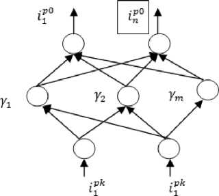
Fig.1. Architecture of KELM network.

Where, P denotes the output weights of the hidden layer, H denotes output matrix of hidden layer and I^{p 0} denotes the desired frontal face image for the given I^pk pose set of specific pose k .

The output weights of the ELM neural network is given by eq. (13).

stability of the KELM regression network, Eq. (14) can be rewritten as eq. (15).

P = H^T( 1 + H Н ^ту ¹ I^p о            (15)

The output function of KELM is given by eq. (16).

у = h(x)P = h(x)H^T ( 1 + HH^Т У ^о    (16)

The kernel matrix is defined based on mercer's conditions from eq. (16) when hidden layer feature mapping h(x) is unknown, as in eq. (17).

^elm = HH^T

Using eq. (17), eq.(16) can be rewritten as:

У = [ k(P^pk , p ^k ), k(P^pk p ^k)..... k( I^pk , Pf ^k)]

(1 + Delm) "" i P p 0(18)

Therefore, KELM regression can be implemented in only single step. The desired frontal image can be estimated by eq. (19).

Ip 0 = k(ip k, Pf У* p(19)

where, is the non linear regression operator and given by eq.(20)

P = ( 1 + D el m ) ~ i p ⁰⁰

Now, for test posed image ipk, the frontal view can be estimated by using eq.

jP 0 =k( p^k, pf ^k)* P

KELM regression can be explained in simple way as: calculate the kernel matrix k(l^{p k}, ^pf^k^ and non linear regression operator for posed test image using eq. (18) and (20) and then finally use eq. (21) to get the final virtual frontal image .

P = H ip^Po

Here, H ¹ denotes the moore-penorse inverse of matrix H . To calculate the inverse of matrix H , the orthogonal projection method is mostly used. According to orthogonal projection method, if HH^T is non singular, H^L is given by eq. (14)

H1 = HT(HHTy1 (14)

The authors in [34] suggested to add the regulation coefficient, R to the term H H^T in the above expression to make the network more stable. Therefore, to improve the

• V.    Experimental Results

In this investigation, GTAV [35] database with pose variations is used to show the performance of the KELM regression to normalize the pose variations for face recognition. This database contain total 44 subjects including 27 pictures per subject with different pose views at pose angles 0º, ±10º, ±20º, ±30º and ±45º. In this study, each subject with 5 poses at angles 0º, +10º, +20º, +30º and +45º is considered. The resolution of each image is 240 x320 and in .bmp format.

A. Virtual Frontal View Generation

In this section, the results of virtual frontal view generation using three different techniques are presented. The virtual frontal views are generated for all the 4 posed view sets. For virtual view generation, each image is resized to 80 x 80 pixels resolution after fixing the position of eyes and maintaining the same aspects of all the faces, and converted into gray scale image. For experiments, 34 subjects of GTAV database are taken for training purpose to calculate non linear regression operator and the rest 10 images are taken for test purpose to normalize pose variations.

Fig. 2. shows the virtual view generation results for the four poses of GTAV database of the same person using three different techniques. These techniques are: (1) linear regression (2) ELM regression and (3) KELM regression. In fig. 2(a)., the first column of Fig. 2. is the non frontal face images of 4 poses whose pose angles varies from +100  to +450. Fig. 2(b). shows the virtual view generation results after using linear regression. Fig. 2(c). is the reconstruction results using ELM regression and Fig. 2(d). shows the results using KELM regression for virtual frontal view generation. In KELM regression, polynomial kernel is used to calculate the hidden layer output as it is computational efficient. The expression for calculating polynomial kernel function is given by eq. (9).

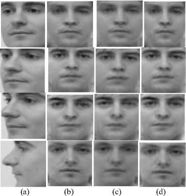
Fig.2. Results of prediction of the virtual frontal view. First column (a) is the input non frontal posed face images. Column (b) is the predicted virtual frontal views by linear regression, column (c) is the virtual frontal view predicted by using ELM regression and column (d) is virtual frontal view generated by KELM regression.

To evaluate the virtual view prediction accuracy, the similarity between virtual predicted image and its corresponding frontal face view, four measures are taken into account. These are: RMSE, Cross Correlation Coefficient, Mean Absolute Error, and Normalized Cross Correlation Coefficient.

RMSE is defined as the square root of the mean or average of square of all of the error between two matrices. RMSE is calculated by using the eq. (22).

RMSE = ^^.D-^.P i_/2

*7        y

where, / 1 ( i, j ) is the true frontal view, and / ₂ (i,j) is the predicted virtual frontal view, and M * N is the size of the image. According to the experimental results, RMSE of the predicted virtual frontal view using three approaches for all the four poses of GTAV database is given in Table 1. Table 1. shows the best results for predicting virtual frontal view on all the pose sets using KELM regression compared to linear regression.

Table 1. RMSE for virtual frontal view prediction using KELM, ELM and linear regression

Pose Set	Linear Regression	ELM Regression	Kernel ELM Regression
02	0.0990	0.0977	0.0896
03	0.0908	0.0890	0.0892
04	0.9440	0.0924	0.0871
05	0.1043	0.0996	0.0972

Cross correlation is the similarity measure of two matrices or measures the degree to which two matrices are correlated. Expression for calculating cross correlation is given by eq. (23).

Corr Coeff

₌    2£ 1 2 7= i (A(ij)-TO(/ 2 ( i,j)-(T^t)

Ж= 1 2 7= i(fi (i.j)-/^)((f 2 (iJ)-(ra

Table 2. shows the cross correlation measures of the predicted virtual frontal view using three approaches for all the four poses of GTAV database. Table 2. also shows the best results for predicting virtual frontal view on all the pose sets using KELM regression compared to linear regression.

Table 2. Cross Correlation for virtual frontal view prediction using KELM, ELM and linear regression

Pose Set	Linear Regression	ELM Regression	Kernel ELM Regression
02	0.7317	0.7287	0.7463
03	0.6223	0.6713	0.6357
04	0.6823	0.7874	0.7057
05	0.6421	0.5709	0.6471

Mean absolute error (MAE) is an average of absolute errors. It is used to measure how output or predicted values are close to the true or target values. The expression for MAE is given by eq. (24).

МАЕ = ^∑ ^i ^| fit ^- /21|= ; ^∑7=i ^| e_t | (24)

Table 3. shows the MAE measures of the predicted virtual frontal view using three approaches for all the four poses of GTAV database. Table 3. also shows the best results on all the pose sets using KELM regression compared to linear regression.

Table 3. Mean Absolute Error for virtual frontal view prediction using KELM, ELM and linear regression

Pose Set	Linear Regression	ELM Regression	Kernel ELM Regression
02	0.1003	0.2086	0.0943
03	0.1334	0.2470	0.1367
04	0.1320	0.3022	0.1303
05	0.1308	0.3295	0.1213

Normalized Cross Correlation computes the normalized cross correlation of two series. This is done at every step by subtracting the mean of the matrix and then dividing by the standard deviation. Expression for normalized cross correlation is given by eq. (25).

1 ( ft ⁽ х , У )- ̅)( /2 ⁽ х , У )- ̅)

Not Cross Corr=∑ nZ—i           ata2

, J

Table 4. shows the normalized cross correlation values of the virtual frontal view using three approaches for all the four poses of GTAV database. Also, Table 4. shows the best results for proposed work of generating virtual frontal view using Kernel ELM compared to linear method.

Table 4. Normalized Cross Correlation for virtual frontal view prediction using KELM, ELM and linear regression

Pose Set	Linear Regression	ELM Regression	Kernel ELM Regression
02	1.0289	0.9569	1.1735
03	0.9300	1.0378	1.2007
04	0.9531	1.0212	1.2769
05	0.9821	1.0057	1.2757

• VI.    Conclusions and Further Recommendations of Work

In this investigation, to improve the pose-invariant face recognition, the nonlinear method for predicting the virtual frontal face from its non-frontal face view is presented. The rotation of a human head is the nonlinear problem in a 3D space. Therefore, linear regression method for generating virtual frontal view under linear assumption could not significantly predict the virtual frontal face image. In this study, kernel ELM based nonlinear regression algorithm is used to achieve better results for pose normalization. Polynomial kernel is used here to calculate the kernel matrix for the output of the hidden layer of ELM network. RMSE measure is used to show the comparison of prediction accuracy using linear and non linear regression. The results proves the efficiency of the KELM regression approach for pose normalization.

In future, other more efficient non linear networks for regression can be explored to significantly normalize pose variations.

Acknowledgment

The authors would like to express their sincere thanks to GTAV face databases.