Predictive and analytical capabilities of macroeconomic models in conditions of crisis economic development (using the example of the QUMMIR model)

Russia’s economic development over the previous 30 years has been characterized by periodic shocks of both economic and non-economic nature. We can recall at least five of the most significant crises that seriously affected the prevailing macroeconomic proportions and required significant adjustments to the parameters of economic policy: the default of 1998 (Drobyshevskii, Kadochnikov, 2003), the global financial crisis of 2008–2009 (Voskoboynikov et al., 2021), the monetary and financial crisis of 2014– 2015 (Dubinin, 2015), the pandemic crisis of 2020, the sanctions crisis of 2022 (Shokhin et al., 2021). Every time during these crises, the question arose about the quality of macroeconomic forecasts and their place in the decision-making system.

As a science, economics is inseparable from calculations. As we know, it is possible to manage qualitatively only those processes that can be measured. At the same time, the criteria for the calculation accuracy applied to the natural sciences cannot be automatically transferred to social processes where experiment is practically impossible and there is no absolute evidence. The behavior of economic agents is a complex process, the description of which can be approached, but as it is fashionable to say now, to have a complete digital double of society is still beyond human capabilities. Due to the noted above, we should unequivocally state that the use of a calculated approach in justifying economic policy can play a key role, but cannot serve as the only proof of the correctness of a particular decision.

However, questions about the quality and accuracy of forecasts are constantly being raised both in the expert community and at the government level (Klistorin, 2011), so it seems important to discuss once again the key principles of developing medium-term macroeconomic models and forecasts based on them. As the material for such an analysis, we chose the quarter macroeconomic model QUMMIR1, which has been developed at the Institute of Economic Forecasting of RAS for a number of years. To date, more than 50 quarterly macroeconomic forecasts have been prepared on its basis, which means that quite a lot of experience has been accumulated in the application of such tools. In addition, at least four economic crises occurred during this period of contemporary Russian history, which also provided a large amount of information about the necessary properties of large macroeconomic models.

Macroeconomic modeling and economic policy

Applied simulation of economic processes became widespread in the 1960s, when, first, a modern methodological base of global statistical observations was formed (Tinbergen, Boss, 1967), and second, a set of econometric and balance approaches to the practical use of mathematical methods in the analysis and forecasting of economic dynamics was developed (DeJong, 2011).

However, in 1976 R. Lucas published an article, where he criticized the use of econometric models for economic policy analysis (Lucas, 1976). By giving concrete examples of the use of econometric models to analyze the effects of tax policy, Lucas proved the impossibility of obtaining adequate results. The criticism given in the article concerned specific examples, in particular the effects of changes in tax policy, as well as the relationship between inflation and unemployment based on the Philips curve. A significant part of economists took this article as proof of the impossibility of analyzing the effects of economic policy using econometric models, although the material presented was absolutely insufficient to prove such a thesis. Moreover, according to the fair remark of C. Almon, any parameter of economic policy can be replaced by an appropriate variable reflecting its functionality (Almon, 2016), which means that the solution to the problem is not to abandon econometrics, but to make econometric dependencies have a clear interpretation and most adequately describe the cause-and-effect relationships that exist in the real economy.

Lucas’ criticism forced many economists to think about the correspondence of the mathematical tools used to the tasks of describing the real economy and led to the development of other methods of economic modeling aimed at describing the economic behavior of economic agents (Shoven, Whalley, 1984; Shoven, Whalley, 1992; Makarov et al., 2022). This direction has given rise to whole classes of models, such as, for example, computable general equilibrium models (CGE) or dynamic stochastic general equilibrium models (DSGE). It is worth saying that from the point of view of forecasting and economic analysis, these models are an accurate response to criticism of using the econometric approach, since they rely on the theory of the real business cycle and try simulating changes in the behavior of economic agents for various macroeconomic shocks. The only problem is that when conducting behavioral modeling, theoretical postulates are used, which do not always correspond to the reality of specific national economies. In this regard, we can say that this class of models contributed to the advancement of economics, but could not replace models that consider cause-and-effect relationships within a particular economy (Hausman, 2011; Bardazzi, Ghezzi, 2021). To solve this problem, it is necessary to work with real data and describe the interactions existing in the economy with the help of econometric dependencies.

Creating an applied econometric model is a complex task requiring considerable time and efforts of qualified specialists. At the same time, this is the best way to understand the features of the functioning of the real economy, especially for young colleagues who are taking their first professional steps in studying the national economy (Almon, 2012). As practice shows, it is better to start introducing students and postgraduates into the complex world of economic interactions with simple macroeconomic calculations describing one or another aspect of economic life: population incomes and expenditures, budget system, foreign trade, etc. However, work on a comprehensive model is a key step for developing the general economic outlook of a specialist who wants to work in the field applied analysis and justification of economic policy. The ability to work with a complex macroeconomic model, form scenarios and modernize the main dependencies create the basis for working on more complex forecasting and analytical structures, including intersectoral ones.

In this regard, the quarter macroeconomic model QUMMIR should be perceived not only as a key predictive tool used for medium-term forecasting in the IEF RAS, but also as an important element of analytical work that allows quickly assessing changes in key factors affecting the economic development.

Quarter macroeconomic model QUMMIR – general description

The model is based on a sequential iterative calculation of forecast indicators of economic dynamics in increments of one quarter. The calculation of the dynamics of macroeconomic indicators is carried out in the logic of demand: population, business and the state. Demand is formed depending on the income level, as well as the structure and volume of savings of economic entities.

Incomes, in turn, are formed on the basis of the economic activity results obtained in accordance with the distribution of demand of economic agents for imported and Russian products, as well as the dynamics of external demand (exports). We assume that the demand for goods and services of Russian production is fully provided by the corresponding supply. In our opinion, such logic of calculation construction is appropriate when modeling the economy’s dynamics in short and medium term. Forecasting indicators over a longer period requires additional consideration of resource constraints, including the volume and structure of capital.

Thus, the model is a closed system in which income, demand, domestic production, imports and prices interact.

Currently, there are more than 2,000 variables in the database and a system of more than 200 equations.

The statistical database of the model contains quarter data series in the following directions:

• 1)    national accounts: GDP produced (since 2003), GDP used (since 1993), GDP by sources of income (since 1995, source: Rosstat);

• 2)    investments in fixed assets by sources of financing (since 2002, source: Rosstat);

• 3)    population income and expenses (since 1995, source: Rosstat);

• 4)    employment statistics (since 1998, source: Rosstat);

• 5)    demographic statistics (since 1996, source: Rosstat);

• 6)    price dynamics (since 1993 deflators of elements of final demand and consumer price indices, source: Rosstat);

• 7)    consolidated budget and budgets of extrabudgetary funds (since 1995, source: Federal Treasury of the Russian Federation, Ministry of Finance of the Russian Federation);

• 8)    indicators of the financial condition of organizations (since the 2nd quarter of 1998, source Rosstat);

• 9)    external sector statistics: balance of payments in analytical representation (since 1994, source: Central Bank of the Russian Federation), ruble exchange rate (to the U.S. dollar since 1993, to the euro since 1999, source: Central Bank of the Russian Federation);

• 10)    foreign trade statistics: exports of energy goods, structure of imports of goods by end-use purposes, export price of natural gas (since 1994, source: Federal Customs Service of Russia);

• 11)    review of credit institutions and the Central Bank (since 1995; source: Central Bank of the Russian Federation);

• 12)    statistics on the activities of fuel and energy companies (since 2005, source: Rosstat, Ministry of Energy of the Russian Federation), price of Urals grade oil (since 1993, source: Ministry of Finance of the Russian Federation);

• 13)    statistics of goods and services markets (from 1993–1995, source: Rosstat);

• 14)    indices of prices of energy resource producers (since 2000), tariffs for railway transportation of goods (since 1997, source: Rosstat);

• 15)    other variables of internal economic activity: minimum wage (since 1993), pension amount (since the 2nd quarter of 2006), new housing supply (since 1998, source: Rosstat);

• 16)    outside world statistics: U.S. GDP, U.S. current account balance (since 1993, source: U.S. Bureau of Economic Analysis), Eurozone GDP (since 1995, source: European Central Bank);

• 17)    world market indicators: Brent oil prices, wheat (since 1993, source: World Bank), U.S. Federal Reserve System discount rate (since 1993, source: U.S. Federal Reserve System).

The model contains GDP calculation by elements of use in current and comparable prices in terms of modeling price dynamics (deflators of elements of final demand). In addition, the account of GDP production in constant prices is modeled.

The model includes a system of balances, which allows limiting the range and increase the “rigidity” of the forecast in the calculation system. They include:

• –    balance of personal income and expenses;

• –    incomes, expenses and budget surplus/ deficit;

• –    balance of payments;

• –    balance of the Central Bank;

• –    balance of credit institutions.

In accordance with the logic of calculation formation, the model is a system of several interrelated blocks, including GDP calculation block; price block; personal income and expenditure block; tax and budget block; investment block; block of balance of payments; financial block; employment block; and energy block.

The main exogenous variables of the model are a set of parameters of the external economic environment, as well as internal factors, mainly related to the parameters of economic policy.

External factors include variables reflecting the external and associated conditions of the functioning of the Russian economy. The complex of external factors can be divided into groups.

• 1.    Global demand for goods and services:

• –    price of Brent and Urals crude oil;

• –    gas price;

• –    dynamics of U.S. and Eurozone GDP;

• –    wheat price.

• 2.    World demand/supply of financial resources:

• –    ratio of world currencies (euro/U.S. dollar);

• –    dynamics of external debt of the Russian private sector (banks and other sectors) in the context of the investment climate/element of geopolitics.

Internal factors include variables reflecting the internal conditions of the functioning of the Russian economy. This group of factors characterizes the Russian policy directions, prices of the infrastructure sector, and describes the demographic situation, certain aspects of enterprises’ activities.

According to the Russian policy directions, we can distribute the factors as follows.

• 1.    Fiscal policy:

  – in terms of budget system revenue generation (tax rates);

  – in terms of requirements for the dynamics of budget expenditures (functional structure of consolidated budget expenditures);

  – from the standpoint of the possibility of attracting sources of financing the budget deficit (the amount of public debt – external and internal, the use of previously accumulated funds of the National Welfare Fund);

• 2.    State social policy: minimum wage; average pension growth index.

• 3.    Monetary policy:

  – ruble exchange rate (actions of the Central Bank of the Russian Federation on the Russian currency market, including within the framework of the budget rule, provision of funds in foreign currency to credit institutions, restrictions on the movement of capital of individuals and legal

entities, standards for the mandatory sale of foreign exchange earnings);

– key rate of the Bank of Russia.

The parameters of the infrastructure sector and demographic situation include the price indices of natural monopolies (electricity, gas, rail transportation) and demographic indicators (population, including those of working age; number of students, pensioners).

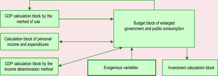
Figure 1 shows the schematic diagram of calculations based on the QUMMIR model.

Forecast calculations within the framework of the quarter macroeconomic model are carried out by the iteration method through the simultaneous

Figure 1. Schematic diagram of GDP calculation by using the QUMMIR model

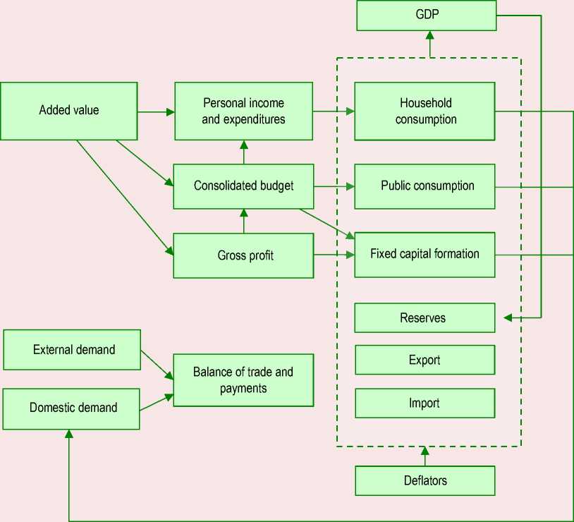
Source: own compilation.

solution of a system of equations with specified accuracy parameters. The convergence criterion is determined for household consumption in such a way that the discrepancy of the calculation results between iterations does not exceed 0.01%.

In turn, scenarios differ in a set of exogenous variables, so the formation and coordination of scenario conditions is a key element of the procedure for predictive calculations.

The model allows making calculations based on scenarios associated with changes in exogenous parameters, including for assessing the effects of various shocks. It is possible to consider both particular scenarios of changes in individual policy directions, and complex scenarios of changes in the situation in the entire economy as a whole.

Estimates of economic dynamics using the QUMMIR model taking into account the ongoing geo-economic changes

The most common option for a medium-term forecast, performed using a quarterly macroeconomic model, is an inertial scenario. Its choice makes it possible to assess economic dynamics in the logic of business as usual in the absence of significant changes in the field of economic policy.

The formation of inertial scenarios is more or less based on the scenario conditions of the Ministry of Economic Development of the Russian Federation, the parameters of the three-year budget and forecast indicators of leading world organizations (International Monetary Fund, World Bank, International Energy Agency).

The value of such a scenario is that it allows assessing the risks of maintaining the current parameters of economic policy in the medium and long term. On the other hand, within the framework of an inertial scenario, it is impossible to implement one of the key goals of forecasting – to justify the economic policy.

This problem can be solved on the basis of assessments of alternative macroeconomic scenarios assuming certain shifts in the parameters of economic policy. The most interesting ones are those in which changes in the parameters of monetary and budgetary policy are assessed, which should be immersed in the general context of the Russian economy development.

The situation developing in the Russian economy after the introduction of new sanctions restrictions in 2022 is characterized by a significant change in the proportions of exchange with the outside world, which inevitably affects the parameters of production, financial and budgetary systems and, in general, the economic dynamics in the country.

According to our estimates, the current crisis features will be the duration of the period of negative GDP dynamics, which will be associated both with restrictions on the supply of imported products and decisions of unfriendly countries to abandon Russian energy carriers and raw materials. In such conditions, a certain period of adaptation of the Russian economy to changes in the structure of production, income and prices will be required. This period will become a necessary condition for the next stage of the Russian economic development – structural and technological restructuring aimed at forming a stable development base in the medium and long term.

In the short term, restrictions related to the unavailability of a number of imported goods will have the most serious impact on the economic dynamics in the country. They will restrain both demand and production, in the part where imported raw materials and components are used. The restoration of import flows, including through the change of suppliers, as well as parallel import mechanisms, will have the greatest impact on the timing of adaptation of the Russian economy to new conditions. We should also take into account that the import of goods is the most significant channel for the receipt of research and development results of developed countries into the Russian economy. Thus, in the medium term, the restrictions imposed on the

Russian economy will directly restrain the growth of production efficiency through restrictions on access to the most effective technological solutions. This situation can be overcome only if investments in research and development are increased, as well as dependence on imports is reduced. It is clear that we are not talking about any form of autarky. Moreover, without building deep cooperative relations in the scientific and technological field with friendly countries, the task of achieving technological sovereignty cannot be solved.

Increasing cooperation with friendly countries will become a natural development of processes in the global economy, where after a period of growth due to globalization processes, a period of slowing down of trade growth and the formation of large regional blocks occurs, which is accompanied by a decrease in the reliability of investments in reserve currencies and the growth of non-tariff barriers to trade. At the same time, the key constraint for developing countries, as before, will remain technological dependence on solutions worked out in developed economies. To change the situation, it is necessary to create an alternative contour of trade and economic relations, which has relative independence from traditional mechanisms of financing, reservation and scientific and technological development.

Technological modernization of the Russian economic development should be supported by appropriate decisions in the field of project financing. In fact, we are talking about a balance between budget and market financing of the directions of structural and technological restructuring of the economy. Here, we should make one important remark – budgetary sources of the economy’s financing are largely limited. For example, the total expenditures of the consolidated budget in 2021 did not exceed 32% of GDP. Accordingly, it will be impossible to rely mainly on the budget channel during the structural readjustment of the economy. At the same time, budgetary resources can become the most important source for launching a new investment cycle, as they allow directing resources to where there are opportunities to achieve the greatest macroeconomic effect, and also demonstrate to business directions for effective investment of funds.

Increasing budget financing requires maintaining a budget deficit for the transition period, which can be financed by internal borrowing. At the same time, it is necessary to comply with a number of conditions: relatively low inflation, definition of the limits of increasing domestic debt. According to our estimates, in the period up to 2025, the benchmark for the level of budget deficit may be up to 3% of GDP, which will not lead to significant damage to the parameters of microfinance stability. It is fundamentally important that irregular budget expenditures related to the structural and technological modernization of the economy should be financed primarily due to the budget deficit.

As for monetary policy, it will play a supporting role when launching a new economic cycle. It is important to maintain a level of the key rate that would not impair the ability of non-financial enterprises to use borrowed resources to finance working capital and investments. However, as economic activity recovers, the role of debt financing will naturally grow, and the role of the banking sector in shaping economic dynamics will increase significantly.

In order to build an active economic policy, aimed at mitigating the negative impact of external restrictions on the Russian economy, it is important to understand the range of influence of key parameters on the formation of economic dynamics. To this end, it is advisable to consider appropriate alternative scenarios.

Before proceeding to the assessment of such scenarios in more detail, let us focus on calculation description in the budget and financial blocks of the QUMMIR model.

Financial block of the model

The purpose of creating a financial block based on the macroeconomic model of Russia is the desire to describe the patterns of development of the monetary sphere in interaction with macroeconomic dynamics. The functioning of the monetary sphere is provided by the country’s banking system, the institutional subjects of which are the Bank of Russia and credit organizations2. Thus, the main task in developing the financial block is to model the performance indicators of banks and the Bank of Russia from the perspective of their internal interaction and relations with other economic entities. As a result, the financial block is represented by interconnected balance sheets of the Central Bank of the Russian Federation and credit institutions, while the connecting elements are the volume of lending to banks from the Central Bank and the requirements of banks to the Central Bank.

Elements of bank balance sheets are calculated taking into account the behavior of the main subjects of the economy: population, organizations, public administration, the outside world – in relation to the formation of savings and borrowing. We use regression analysis to model relationships. The independent variables of the financial block are either endogenous, i.e. calculated within the framework of other blocks of the model, or exogenous – set from the outside.

Personal deposits are modeled depending on wages, incomes, prices and exogenously set exchange rate of the ruble and the structural share of cash in circulation as part of the money supply. Deposits of financial and non-financial organizations are modeled depending on GDP at current prices, turnover of organizations, and exchange rate. Personal loans are calculated depending on incomes and prices, exogenous loan rates and the exchange rate. In addition, exogenous variables of loan terms by type of loans are used to estimate the volume of payments to the population for repayment of credit debts, when modeling housing loans, exogenous indicators of the volume of new housing supply and housing loan rates are used, when calculating car loans, the specified share of passenger car sales in retail trade turnover and the loan rate are used. The dynamics of loans and other requirements to organizations are influenced by the volume of GDP at current prices, the available resources of the banking system, the price level and exchange rate, the rate on loans to organizations calculated depending on the level of a given key rate.

Deposits and other attracted funds of public administration authorities in the banking system are calculated taking into account the balances on the accounts of the expanded government at the beginning of the period, income and expenses of the consolidated budget, volume of external and internal sources of financing of the budget surplus/ deficit. The dynamics of banks’ requirements to government authorities is determined by an exogenously set volume of net issuance of government securities on the domestic market.

The external assets and liabilities of banks depend on the exogenously specified structure of their constituent elements and foreign trade volume.

The requirements of banks to the Central Bank are modeled on the basis of the amount of funds raised, mandatory reserve standards, the key rate, and the price level. This indicator, together with cash in circulation, represents the monetary base in a broad definition, which, along with public funds in the Central Bank, forms the economy’s demand for money. The assets of the Central Bank provide the supply of monetary liquidity, the main components of assets are international reserves and loans and other requirements to banks from the Central Bank. The dynamics of the Central Bank’s requirements for non-residents is determined by exogenous indicators – changes in foreign exchange reserves (including as a result of operations), the volume of monetary gold and the exchange rate. Lending to

Figure 2. Scheme of calculation of balance sheet items of credit institutions

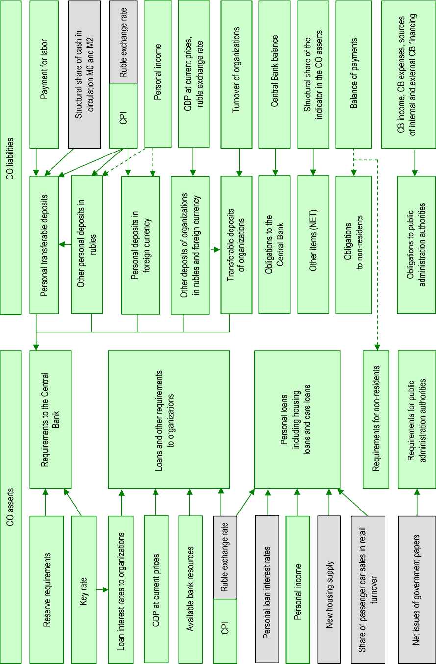
Source: own compilation.

Figure 3. Influence of monetary indicators on other variables of the model

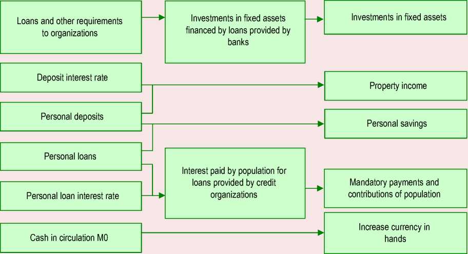
Source: own compilation.

banks is a balancing item in conditions of equality of assets and liabilities of the Central Bank.

The scheme presented in Figure 2 reflects the impact of various macro variables on monetary indicators in the framework of calculating the balance of credit institutions. Here, we separately highlight external variables of the monetary block, including exogenous model variables (gray blocks).

The influence of monetary variables on the forecast of macroeconomic dynamics is carried out through consumer and investment demand by embedding them into the equations of the elements of the balance of population income and expenditure and investments in fixed assets (Fig. 3). For instance, the increase in population deposits minus the increase in credit debt is an integral part of population savings, cash dynamics in circulation determines the increase in cash by currency in hands. The volume of accumulated credit debt, along with loan rates, allows estimating the volume of mandatory payments of the population in relation to the interest paid on loans. Accrued interest on deposits calculated from the volume of population deposits and the deposit rate level are used in modeling property income. Loans and other requirements to organizations are taken into account when calculating the investment volumes in fixed assets financed by loans provided by banks.

Budget block of the model

The described block of the model makes it possible to predict the revenues and expenditures of Russia’s consolidated and federal budgets, the value of which determines public consumption volume and public investment amount in the economy, and also affects the amount of monetary income through the salaries of public sector workers and social transfers. In addition, the block implements the calculation of indicators of budgets of extra-budgetary funds.

The block diagram is as follows:

• 1)    income indicators from basic taxes are calculated (divided into oil and gas and other), the total amount of budget revenues is estimated;

• 2)    volumes of attraction and repayment of internal and external public debt, as well as the structure of consolidated budget expenditures (as elements of budget policy) are exogenously set;

• 3)    indicators of consolidated budget expenditures are projected (through the balance sheet identity of expenditures = revenues + sources of deficit/surplus financing);

• 4)    state consumption volume is calculated in constant and current prices, as well as the investment volumes at the expense of budgetary funds.

The main part of the budget revenues are tax revenues, so the main place in the budget block is occupied by modeling and forecasting of receipts for basic taxes.

At the same time, the model implements separate simulation of oil and gas (mineral extraction tax, export duties, additional income tax, and excise tax on oil refining) and non-oil and gas revenues. As part of the latter for taxes that have a basic tax rate (VAT, income tax, personal income tax, insurance premiums for compulsory social insurance), the income is calculated using econometric equations of the following type:

Amount of tax receipts = taxable base x main nominal rate x estimated level of collection (calculated by the regression equation).

For taxes with no single tax rate, such as excise taxes, the tax base is used as the main explanatory variable. In addition, where possible, exogenously set average dynamics of rates are applied (for example, for excise taxes on tobacco products and alcohol) (Savchishina, 2008).

Thus, the main task in modeling tax revenues is to determine the tax base as correctly as possible.

The main relationships within the fiscal block are reflected in Figures 4, 5 (exogenous parameters are marked with thickened frames).

Figure 4. Budget and state consumption block

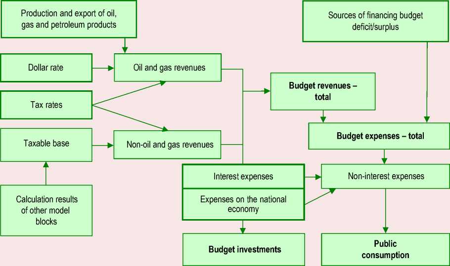
Source: own compilation.

Figure 5. Relationships with other model blocks

Source: own compilation.

To determine the dynamics of exogenous parameters (in particular, sources of budget deficit financing), we use the relevant parameters of the Federal budget law (for the next three years), the explanatory note to which traditionally contains the main parameters of both regional budgets and budgets of extra-budgetary funds3. However, in conditions of high uncertainty, which is typical for crisis periods, the dynamics and structure of budget expenditures become decisive when balancing the forecast (Klepach, 2020). In this case, the research task is to determine, on the one hand, the amount of additional sources of deficit financing necessary to maintain general economic dynamics, and on the other hand, the amount of additional sources of deficit financing that is safe from the point of view of budgetary stability.

Results of forecast assessments

The current economic situation imposes increased requirements on the configuration of the budget system, the stability of which, due to the resulting restrictions, has decreased for objective reasons (Klepach, 2022). The need to fend off external challenges that arose in 2022 led to the formation of a deficit budget. 2023 will be even more difficult from the point of view of budget balance. Next, we will consider the basic forecast of economic development for the medium term, reflecting the authors’ view.

Against the background of a likely decrease in budget revenues by 11% year-on-year in 2023 (including income tax – by 19%, VAT – by 2%, export duties – by 41%, mineral extraction tax – by 21%), even a drop in spending by 4% will require additional financing of a deficit of 4.3 trillion rubles, which is comparable to the situation of the “covid” year of 2020. In the medium term, even a minimal increase in spending (+5% in 2025 to the level of 2021 in nominal terms) against the background of low dynamics of economic recovery will lead to budget execution with a deficit of at least 2 trillion rubles annually until at least 2026–2027. At the same time, the state has the resources to finance such a deficit, primarily through the use of the liquid part of the National Wealth Fund (NWF) and the resumption of limited domestic borrowing ( Tab. 1 ).

However, the budget will be unable to make a significant contribution to the economic dynamics while maintaining the current budget policy (including the resumption of the budget rule) after 2023. After a period of growth in public investment (+5% in 2022 and +2% in 2023 in real terms) and

Table 1. Sources of financing the budget deficit (inertia scenario), trillion rubles

Sources of financing of the CB deficit 2022 2023 2024 2025 Deficit -0.9 -4.3 -1.8 -2.0 Net issue of government papers -1.2 2.0 2.0 2.0 Net external borrowing -0.4 -0.3 -0.3 -0.3 Use of accumulated funds of the NWF 1.8 2.0 0 0 Other 0.7 0.6 0.1 0.3 Source: own compilation .

public consumption in the next two years in 2024– 2025, their real dynamics is highly likely to be zero, and the contribution of public sector to the personal income growth (pensions and salaries of civil servants) will also decrease.

The tools of the QUMMIR model allow considering a number of alternative scenarios, the results of which can be used to justify changes in budget policy. In particular, two factors can be considered:

• •    increase in oil and gas budget revenues due to the weakening of the ruble with conservative spending dynamics;

• •    intensification of economic growth with easing of fiscal and monetary policy.

Calculations under the first scenario show that even a significant weakening of the ruble does not solve the problems of the budget system. For example, in the conditions of 2023, the weakening of the ruble to the level of 90 rubles/USD on average per year would allow for such an increase in oil and gas revenues which would lead to a deficit-free budget. The average annual rate of 82 rubles/ USD will make it possible to execute a budget with a deficit of no more than 2 trillion rubles, for which there are enough internal loans to finance; it means that the preservation of the NWF volume will be ensured. However, with both variants of the weakening of the national currency, the general economic situation worsens. The dynamics of those elements of domestic demand directly financing by the state (state investments and state consumption) will be slightly lower than in the inertial scenario (by 0.8 and 0.1 percentage points, respectively) due to rising prices.

The greatest losses will be recorded for businesses and population ( Tab. 2 ). Even with the real income growth, a reduction in imports against the

Table 2. Results of alternative scenarios for 2023

Macroeconomic results of 2023	Inertial scenario	Ruble weakening scenario	Scenario for saving budget expenditures
GDP, % to the previous year	-1.5	-1.5	-1.2
Household consumption, % to the previous year	-1.3	-3.2	-0.6
Investments, % to the previous year, including:	-1.3	-3.0	-1.0
state	+2.1	+1.3	+3.0
in fuel and energy sector	-1.3	-5.0	-1.3
other private investments	-1.9	-3.4	-1.8
Import, % to the previous year, including:	+1.3	-6.2	+1.7
consumer	-3.4	-18.5	-2.4
investment	+1.1	-9.5	+1.2
Consolidated budget revenues, trillion rubles	41.4	43.6	41.4
expenses	45.7	45.7	47.7
deficit	-4.3	-2.1	-6.2
Inflation, %	5.4	6.5	5.4
Source: own compilation.

background of the appreciation of dollar will significantly reduce household consumption and investment (both in the fuel and energy sector and in other activities).

The results of the budget policy easing scenario look more positive. If the consolidated budget expenditures remain at the level of 2022 in 2023, it will be possible to carry out an increased indexation of pensions and the minimum wage (by 10% vs 6% in the inertial scenario), which will increase the dynamics of real population incomes (from +2.3% in the baseline scenario to +3%) and consumption, and after that – investments (however, in a much smaller volume). At the same time, we do not expect any significant acceleration of inflation in the conditions of a stable exchange rate. The total GDP growth in 2023–2025 will amount to 1.6 trillion rubles regarding the inertial scenario. Nevertheless, without the restoration of production chains disrupted by sanctions, short-term fiscal policy easing alone is not enough for truly active economic growth.

Now let us try assessing the impact of the parameters of the scenarios under consideration on financial indicators, in particular when the parameters of the ruble exchange rate change.

In the forecast for the inertial scenario, personal savings in the form of bank deposits in rubles increase by +3.9–4.5% of income annually in 2022–2025. Deposits of organizations are increasing by +2.9–2.7% of GDP in 2022–2023 and +1.6% of GDP in 2024–2025. This dynamics determines the growth rate of the M2 money supply at the level of +10.3% YoY in 2023, followed by a decrease to +8.3% YoY and +7.3% YoY in 2024–2025. The volume of money supply M2 to GDP at the same time increases from 50.6% at the beginning of 2022 to 60.9% by the end of 2025. Assuming the absence of operations on reserve assets and the preservation of the monetary gold volume, the role of lending to banks by the Central Bank in providing the economy with liquidity is gradually increasing. The volume of the Central Bank’s requirements to banks in 2023–2025 is in the range of 6.5–9.7 trillion rubles and is comparable to the level of 2014– 2015. Deposits of the government authorities in the Central Bank are declining in conditions of budget deficit, the monetary base in a broad definition is increasing at a rate of +13% – +5.4 YoY in 2023–2025 and by the end of the forecast period reaches half in the structure of the Central Bank’s liabilities. Household lending is increasing at a rapid pace +11.2 – +13.9 % YoY in 2023–2025, which makes it possible to maintain consumer spending at the level of 78.2–81.2% of the total population income. The increase in the banks’ requirements to organizations is in the range +7.8 – +8.8 % YoY in 2023–2025, while the investment volume in fixed assets financed by borrowed loans from banks is estimated at 2.1–2.3 trillion rubles annually.

In general, within the framework of the inertial scenario of the Russian economic development, there is a gradual recovery in the level of lending to the population and non-financial enterprises.

In the forecast for the alternative scenario with the weakening of the ruble in 2023, an important factor is the acceleration of price dynamics in comparison with the inertial option. The concomitant additional increase in rates has a restraining effect on household lending– the increase in debt in 2023 is reduced to +8.1% YoY. Personal savings, on the contrary, turn out to be higher in comparison with the inertial option – as a result, the share of consumer spending decreases to 76.8% of total income, and real household consumption decreases more intensively (-3.2%). The dynamics of requirements for organizations in this variant is slightly higher (+10.2% YoY), but at the same time, investments in fixed assets financed by loans provided by banks, while maintaining the nominal volume, are declining in real terms in 2023 at a high rate (-7.7 and -3.6%, respectively, according to the options) in conditions of an increase in the price level.

Based on the above calculations, we can conclude that in the current conditions in the Russian economy, a significant weakening of the ruble exchange rate no longer plays the same stabilizing role as in the previous two decades. The factor of maintaining the competitiveness of Russian exporters remains significant; however, in the conditions of external restrictions, serious changes are taking place here.

Conclusion

In conclusion, we can note that the use of complex econometric macroeconomic models remains one of the most effective tools for justifying regular economic policy, which, on the one hand, solves the problems of studying the mechanisms of forming economic dynamics at the macro level, and on the other hand, not only allows making complex calculations of economic dynamics, but also assessing the effectiveness of individual economic policy measures.

All of the above does not mean that econometric macro modeling is a universal way to justify decisions in the field of economic policy in the medium term. At the same time, given the description of key interactions in the economy and the use of existing data sets, it can become an important argument in the discussion about improving the effectiveness of macroeconomic policy.