Quantum supremacy in end-to-end intelligent IT. Pt. 2: state - of - art of quantum SW/HW computational gate-model toolkit

Quantum computation explores the possibilities of applying quantum mechanics to computer science. If built, quantum computers would provide speed-ups over conventional computers for a variety of problems. The two most famous results in this area are Shor’s quantum algorithms for factoring and finding discrete logarithms, and Grover’s quantum search algorithm show that quantum computers can solve certain computation problems significantly faster than any classical computers. Shor’s and Grover’s algorithms have been followed by a lot of other results. Each of these algorithms has been generalized and applied to several other problems.

The difference between classical and quantum algorithms (QA)s is following: problem solved by QA is coded in the structure of the quantum operators. Input to QA in this case is always the same. Output of QA says which problem was coded. In some sense, you give a function to QA to analyze and QA returns its qualitative property as an answer without quantitative computing. Thus, QA studies qualitative properties of the functions. In these series of scientific articles of quantum software engineering, we concentrate our attention on quantum software and hardware engineering approaches for solution search of intractable classical tasks from computer science, intelligent information technologies, artificial intelligence, classical and quantum control. Many solutions are received as new decision-making results of developed quantum engineering IT and have important scientific and industrial applications [1, 2].

Various traditional models of computing have been generalized to the quantum setting as the models of quantum computing, including quantum Turing machines (QTMs) and quantum circuits. Several novel quantum computing models that have no classical counter-parts have also been proposed, e.g. measurementbased and one-way quantum computing, adiabatic quantum computing etc. Furthermore, the relationships between these models have been thoroughly studied.

Quantum Random Access Machines. Random access machines (RAMs) and random access stored-program machines (RASPs) are another model of computing that is closer to the architecture of real-world computers than Turing machines (TMs). They are also convenient in complexity analysis of algorithms. The notion of quantum random access machine (QRAM) was first introduced as a basis of the studies of quantum programming. Essentially, it is a RAM in the traditional sense with the ability to perform a set of quantum operations on quantum registers, including: (1) state preparation, (2) certain unitary operations, and (3) quantum measurements. Recently, several quantum computer architectures have been proposed based on the QRAM model with some practical quantum instruction sets, including IBM OpenQSAM, Rigetti’s guil and Delft’s eQASM.

Today’s High-Performance Supercomputers operate in PetaFLOPS (1015) which is still not enough to meet the requirements for many scientific computing applications. These employ complex distributed architecture of compute units, but nevertheless, are based on (mostly) CMOS technology. The current state of the art transistor gate-length fabrication sizes have reached 14nm based on FinFET technology. As we proceed towards the limits of miniaturization of transistor gate lengths, quantum effects start to emerge rendering the correct transistor functioning no longer possible. This raises scientific curiosity towards ‘the next big revolution’ in computing and thus, emerges an active interest to look into Beyond-CMOS technologies. Quantum Computing is one such highly investigated fields of research that rethinks computing methodology at most fundamental levels by employing quantum effects of ‘superposition’ and ‘entanglement’ to solve classically intractable problems.

A full-stack quantum accelerator . Implementing a quantum algorithm on actual quantum hardware requires several steps at different layers of abstraction. To further complicate the picture, when it talk about quantum computing - talk about several different paradigms. Some of these paradigms are barely abstracted away from the underlying physical implementation, which increases the difficulty of learning them for a computer scientist or a software engineer. Usually define four paradigms:

• 1.    Discrete variable gate-model quantum computing . This is the generalization of digital computing where bits are replaced by qubits and logical transformations by a finite set of unitary gates that can approximate any arbitrary unitary operation. A classical digital circuit transforms bit strings to bit strings through logical operations, whereas a quantum circuit transforms a special probability distribution over bit strings— the quantum state—to another quantum state. Most quantum computing hardware companies focus on this model. For short, we refer to this model as the discrete gate model .

• 2.    Continuous variable gate-model quantum computing . The qubits are replaced by qumodes, which take continuous values. Conceptually this paradigm is closer to the physics way of thinking about quantum mechanics, and quantum optics in particular. Most of the language that describes these circuits uses the terminology of quantum optics. We will refer to this model as the continuous gate model .

• 3.    Adiabatic quantum computation. Quantum annealing devices exploit this model. At a high level, this paradigm uses a phenomenon from quantum physics known as the adiabatic theorem to find the global optimum of a discrete optimization problem. Recently, the actual physical devices that implement this paradigm have also been found useful in sampling a Boltzmann distribution. This paradigm does not have a direct classical analogue, and some understanding of statistical physics is recommended to work in this paradigm. This model will be referred to as quantum annealing .

• 4.    Quantum simulators. These are application-specific quantum devices that are used, for instance, to study a particular model in quantum many-body physics. While this idea was the original motivation behind quantum computing, the field evolved significantly over the last three decades, and due to the lack of generality of this paradigm, we exclude it from our survey. Quantum simulators are not to be confused with simulations of quantum computation on classical computers.

It remains challenging to understand what kind of problem can be solved efficiently by which paradigm and corresponding quantum algorithm. A typical quantum algorithm workflow on a gate-model quantum computer is shown in Fig 1a, whereas Fig 1b shows a typical workflow when using quantum annealing.

Both start with a high-level problem definition such as e.g. ‘solve the Travelling Salesman Problem on graph X ’. The first step is to decide on a suitable quantum algorithm for the problem at hand. We define a quantum algorithm as a finite sequence of steps for solving a problem whereby each step can be executed on a quantum computer. In the case of the Travelling Salesman Problem we face a discrete optimization problem.

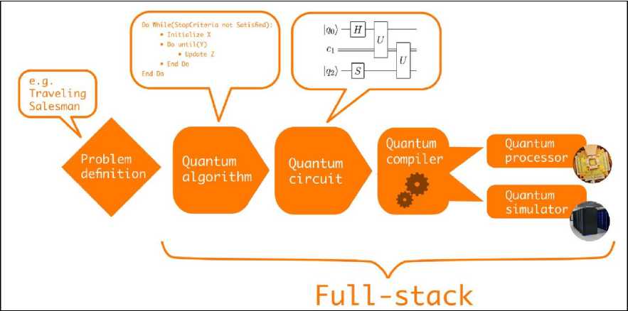
Fig 1a. Visualization of a typical quantum algorithm workflow on a gate-model quantum computer

First, the problem is defined at a high-level and based on the nature of the problem a suitable quantum algorithm is chosen. Next, the quantum algorithm is expressed as a quantum circuit which in turn needs to be compiled to a specific quantum gate set. Finally, the quantum circuit is either executed on a quantum processor or simulated with a quantum computer simulator.

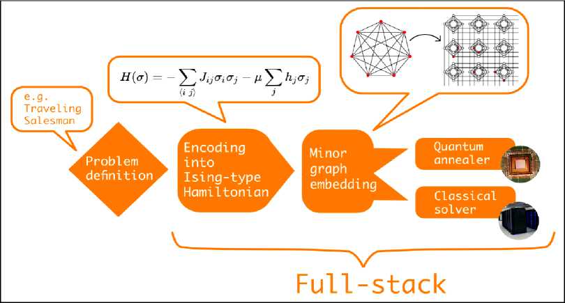
Fig 1b. Visualization of a typical quantum algorithm workflow on a quantum annealer

First, the problem is defined at a high level and is then encoded into an Ising-type Hamiltonian which can be visualized as a graph. Next, via minor graph embedding the problem Hamiltonian needs to be embedded into the quantum hardware graph. Finally, either a quantum annealer or a classical solver is used to sample low-energy states corresponding to (near-)optimal solutions to the original problem.

Thus, the user can consider e.g. the quantum approximate optimization algorithm that was designed for noisy discrete gate model quantum computers or quantum annealing to find the optimal solution. Some of the open source projects require the user to define the quantum circuit of gates manually that represents the chosen algorithm for the given problem definition and quantum computing paradigm. Other projects add another level of abstraction by allowing the user to simply define the graph X and a starting point A, which encapsulates the Travelling Salesman Problem, and then automatically generate the quantum circuit for the chosen algorithm.

Note, that we explicitly distinguish a quantum algorithm from a quantum circuit. A quantum circuit is a quantum algorithm implemented within the gate-model paradigm whereas our notion of a quantum algorithm also includes the quantum annealing protocol.

If the scale of the quantum system is still classically simblable, the resulting quantum circuit can be simulated directly with one of the available open source quantum computer simulators on a classical computer. The terminology is confusing, since hardware-based quantum simulators form a quantum computing paradigm as we classified above. Yet, we also often call classical numerical algorithms quantum simulators that model some quantum physical system of interest, for instance, a quantum many-body system. To avoid confusion, we will always use the term quantum computer simulator to reflect that a quantum algorithm is simulated on classical hardware. As opposed to a quantum computer simulator, the quantum processing unit (QPU) is the actual quantum hardware representing one of the quantum computing paradigms.

QPUs and some simulators usually only implement a restricted set of quantum gates which requires compilation of the quantum circuit. Compilation connects the abstract quantum circuit description to the actual hardware or the simulator: it is the process of mapping the quantum gate set G in a quantum circuit C to a different quantum gate set G ^∗ resulting in a new quantum circuit G ^∗ . As an intuitive example, many quantum circuits use two-qubit gates between arbitrary pairs of qubits, even though those qubits might not be physically connected on the quantum processor. Hence, the quantum compiler will swap qubits with each other until the required two qubits are neighbors, so the desired two-qubit gate can be implemented. After applying the two-qubit gate we need to reverse the swaps to restore the original configuration. The swaps require several extra gates. For this reason, quantum circuits often increase in depth when being compiled.

The different steps in the quantum algorithm workflow outlined above mostly refer to the (continuous and discrete) gate models. However, useful analogies can be made for the quantum annealing paradigm. As shown in Fig 1b, having chosen quantum annealing as the quantum algorithm to tackle the Traveling Salesman Problem, the next step is to construct an Ising-type Hamiltonian that represents the problem at hand. This is equivalent to constructing a discrete quantum circuit in the gate-model. The actual QPU that performs the annealing seldom corresponds to the interaction pattern of the Hamiltonian. For instance, the quantum annealing processors produced by D-Wave Systems currently have a particular graph topology—the so called Chimera architecture—that has four local and two remote connections for each qubit. Thus, the previously generated problem graph must be mapped to the hardware graph by finding a minor graph embedding. Finding the optimal graph minor is itself an NP-hard problem, which, in practice, requires the use of heuristic algorithms to find suitable embeddings. Finding a graph minor is analogous to quantum compilation and the size of the graph minor can be seen as the direct analogue to quantum circuit depth in the gate-model paradigm. In-depth analyses of quantum annealing performance have revealed a clear dependence between the quality of minor graph embeddings and QPU performance.

Lastly, the embedded graph can either be solved on a QPU or with a classical solver. The latter is similar to using a quantum computer simulator in the gate-model paradigm. When obtaining samples from a quantum annealer, it is common to further postprocess the results with classical algorithms to optimize solution quality. In both the gate-model and annealing paradigm, we define a full-stack library as software that covers the creation, compilation / embedding, simulation and execution of quantum instructions as illustrated in Figs 1a and 1b.

Open source software in quantum computing covers all paradigms and all stages of expressing a quantum algorithm. The software comes in diverse forms, implemented in different programming languages, each with their own vocabulary, or occasionally even defining a domain specific programming language. However, to provide a representative, but still useful study of quantum computing languages and libraries, we limited ourselves to projects that satisfy certain criteria.

Quantum computing simulators

Quantum++ is a high-performance simulator written in C++. Most quantum computer simulators only support two-dimensional qubit systems whereas this software library also supports the simulation of more general quantum processes. Qrack is another C++ based simulator that comes with additional support for Graphics Processing Units (GPUs). The developers of Qrack put special emphasis on performance by supporting parallelization over multiple CPU or GPU cores. A more educational and less performance-oriented quantum computer simulator is Quirk. It is a JavaScript-based simulator that can simulate up to 16 qubits in a modern web browser. Quirk provides a visual user experience by allowing beginners and experts to construct quantum circuits via simple drag-and-drop operations (see Table 1).

Table 1. Overview of projects

Name	Tagline	Programming language	Licence	Supported OS
Cirq	Framework for creating, editing, and invoking Noisy Intermediate Scale Quantum (NISQ) circuits.	Python	Apache-2.0	Windows, Mac, Linux
Cliffords.jl	Efficient calculation of Clifford circuits in Julia.	Julia	MIT	Windows, Mac, Linux
dimod	Shared API for Ising/quadratic unconstrained binary optimization samplers	Python	Apache-2.0	Windows, Linux, Mac
dwave-systen	Basic API for easily incorporating the D-Wave system as a sampler in the D-Wave Ocean software stack	Python	Apache-2.0	Linux, Mac
FenniLib	Open source software for analyzing fermionic quantum simulation algorithms.	Python	Apache-2.0	Windows, Mac, Linux
Forest (pyQuil & Grove)	Simple yet powerful toolkit for writing hybrid quantum-classical progyams.	Python	Apache-2.0	Windows, Mac, Linux
OpenFermion	The electronic structure package for quantum computers.	Python	Apache-2.0	Windows, Mac, Linux
ProjectQ	An open source software framework for quantum computing.	Python, Ch	Apache-2.0	Windows, Mac, Linux
PyZX	Python library for quantum circuit rewriting and optimisation using the ZX-calculus.	Python	GPL-3.0	Windows, Mac, Linux
QGL.jl	A performance orientated QGL compiler.	Julia	Apache-2.0	Windows, Mac, Linux
Qbsolv	Decomposing solver that finds a minimum value of a large quadratic unconstrained binary optimization problem by splitting it into pieces.	c	Apache-2.0	Windows, Linux, Mac
Qiskit Terra 6 Aqua	Quantum Information Science Kit for writing experiments, programs, and applications.	Python, Ch	Apache-2.0	Windows, Mac, Linux
Qiskit Tutorials	A collection of Jupyter notebooks using Qiskit.	Python	Apache-2.0	Windows, Mac, Linux
Qiskit.js	Quantum Information Science Kit for JavaScript	JavaScript	Apache-2.0	Windows, Mac, Linux
Qrack	Comprehensive, GPU accelerated framework for dewloping universal virtual quantum processors.	C++	GPL-3.0	Linux, Mac
Quantum Fog	Python tools for analyzing both classical and quantum Bayesian networks.	Python	BSD-3-Clause	Windows, Mac, Linux
Quantum++	A modem C++1 1 quantum computing library.	Ch-, Python	MIT	Windows, Mac, Linux
Qubiter	Python tools for reading, writing, compiling simulating quantum computer circuits.	Python, Ch	BSD- 3-Clause	Windows, Mac. Linux
Quirk	Drag-and-drop quantum circuit simulator for your browser to explore and understand small quantum circuits.	JavaScript	Apache-2.0	Windows, Mac, Linux
reference-qvm	A reference implementation for a Quantum Virtual Machine in Python.	Python	Apache-2.0	Windows, Mac, Linux
ScaffCC	Compilation, analysis and optimization framework for the Scaffold quantum programming language.	C++, Objective G LLVM	BSD 2-Clause	Linux, Mac
Strawberry Fields	Full stack library for designing simulating and optimizing continuous variable quantum optical circuits.	Python	Apache-2.0	Windows, Mac, Linux
XACC	eXtreme-scale Accelerator programming framewoik	Ch	Eclipse PL1.0	Windows, Mac, Linux
XACC VQE	Variational quantum eigensolver built on XACC for distributed, and shared memory systems.	C++	BSD 3-Clause	Windows, Mac, Linux

Next, Rigetti Computing, a hardware startup focused on superconducting circuits for the discrete gate model, has open sourced the project reference-qvm. This is a Open source software in quantum computing reference implementation of the Quantum Virtual Machine (QVM), synonymous with quantum computer simulator, used in their full-stack library Forest. It is a purely Python-based simulator which is meant for rapid prototyping of quantum circuits. So far, all mentioned quantum computer simulators simulate any quantum circuit until a certain depth. This implies that these simulators support Clifford as well as nonClifford quantum gates. In contrast, the project Cliffords.jl restricts itself only to quantum gates from the Clifford group. It is widely known that Clifford circuits can be simulated efficiently with a classical computer and Cliffords.jl allows for fast and efficient calculations by making use of the tableau representation and it is written in the high-performance programming language Julia.

All quantum computer simulators so far are focused on the simulation of gate-model quantum computers. Most of these simulators are used to develop and test quantum algorithms before implementing them on actual quantum chips or to verify results obtained from a QPU. Analogously, the project Qbsolv is used to develop and verify the results obtained from quantum annealing devices. Technically, it is not a quantum computer simulator as previously defined since it uses a classical algorithm unrelated to the physics of quantum annealing.

Yet, we are including it in this discussion because it is the closest analogue to a simulator for quantum annealing devices. It is a C library that finds the minimum values of large quadratic unconstrained binary optimization (QUBO) problems. To achieve this, the QUBO problem is first decomposed into smaller problems which are then solved individually using tabu search, a metaheuristic algorithm based on local neighbourhood search.

The concept of accelerator technology originates from the idea that any end-application contains multiple parts, and the properties of these parts are better executed by a particular accelerator (such as, FPGA, GPU, DSP, TPU etc). This is shown in Fig. 1c.

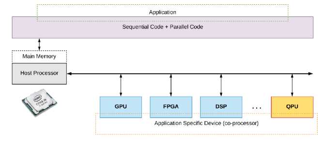
Fig. 1c. System architecture with heterogeneous accelerators

An accelerator has a co-processor (Device) communicating to a central processor (Host). The Device executes certain parts of the overall application much faster than the Host. Similarly, quantum processors are good at solving certain parts of the problem that are inefficient to be solved by classical processors. Furthermore, the quantum assembly language allows user to specify the complete quantum algorithm - containing both classical computational elements and a ‘quantum kernel’. The classical processor keeps the control over the total system and delegates the execution of certain parts to the present accelerators. The functioning of such an accelerator requires abstracting away the low-level (qubit technology) details from the algorithm developer and integrate the software (programming language and compiler) to the hardware (qubit control electronics, cryogenic electronics and qubits themselves).

Given the proposition of Noisy Intermediate-Scale Quantum technology (NISQ), the Quantum Processing Unit (QPU) would prove to be elemental in accelerating calculations for numerous applications such as, simulation of molecules, Protein Folding, Genome Sequencing, Quantum Field Theory simulations, Quantum Machine Learning and many others. In order to execute complex algorithms, we require a system architecture connecting quantum circuit descriptions to the low-level pulses that operating on the physical qubits.

Figure 2 is such an example of a «full-stack» system architecture developed by the Quantum Computer Architecture Lab in Delft.

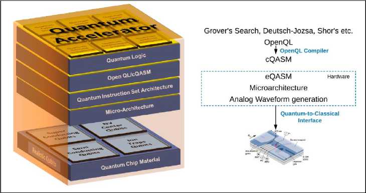
Fig. 2. QCA Lab’s Full-Stack Quantum Accelerator

The quantum compilation tool chain consists of the OpenQL compiler, that translates circuit-level algorithmic descriptions and high-level quantum and classical libraries (for example, QFT, classical optimizers etc.) to a Quantum Assembly Language (cQASM) description, a low-level compiler translates the cQASM description to a platform-independent Quantum Instruction Set Architecture (QISA). The QISA layer contains both classical and quantum instructions. The micro-architecture layer constitutes the implementation of QISA, and is responsible for translating the eQASM instructions to analog waveform with precise timing specifications while being synchronous with multiple channels. The Quantum-to-Classical layer forms comprises of a analog electronic devices that is the interface for analog signals to act upon the physical qubits on the Quantum Chip.

The objective of this approach is directed towards addressing the architectural challenges for the quantum-classical hardware for controlling the NISQ-era quantum devices and beyond. We take into account two of the promising circuit-model based quantum technologies of the future namely, superconducting qubits and Spin-qubits in Quantum-dot, analyze the control infrastructure requirements and propose a microarchitecture to integrate the physical device with the quantum compilation tool chain.

The architecture prototype is developed on a SoC-FPGA platform in the form of a central-controller hardware, CC-Spin. The current version is targeted towards Spin-Qubit in Quantum Dot technology (hereafter referred to as, "Spin-qubit quantum processor"). The central controller interfaced to modular AWG units perform the waveform generation such that, the number of DAC channels scale linearly with the number of AWG-modules on the central controller. The results of the micro-architecture are presented as wave form generations applicable to Spin-Qubit achieved on an oscilloscope, thereby validating the applicability of the architecture to a Spin-qubit quantum processor. Towards the end, we analyze the scalability of such an architecture based on the parameters of number of channels, channel capacity and ability to be integrated as an ASIC. The integration of such a micro-architecture is relevant not only to theorist and programmers but to the experimentalist as well. The micro-architecture reduces the high-resource consumption, reduces the control complexity, and allows faster prototyping and execution of experiments.

In practical systems, a qubit is a physical object and is realized through different physical quantum mechanical systems. The Micro-architecture layer is the interface between the high-level programming infrastructure and the low-level signal generation systems. This layer is interfaced to the qubits (at the Physical layer) via quantum-classical interface. Now we will introduce topics on control of two of the prominent technologies for realizing qubits, namely, Spin-Qubit in Semiconductor Quantum Dot and Superconducting Transmon Qubits.

Spin-qubits in quantum dots. Quantum computing emerged from the idea that quantum degrees of freedom can be utilized to encode and process information. This led the researchers to investigate ideas of fabrication, addressing and manipulation of single-quantum system, that could help in realization of the quantum computer. Today, we have many ways to realize single-quantum systems that can be used to encode qubits, however the challenge to solid-state quantum computation lies in eliminating unwanted noise, arising due to interaction of the qubit with the environment and/or the host material.

Spin Qubits, first proposed in 1997, is one of the Solid-state quantum computing methods that uses spins of electrons confined in quantum dots. For quantum dot-based qubits, the charge and nuclear spin noises lead to decoherence and gate errors. It has been demonstrated that these noises can be tackled by dynamical decoupling and decoherence free subspaces. Noise can further be reduced and coherence time extended to seconds by growing better oxides and heterostructures, and by fabricating the spin qubit in Silicon (28Si), reason being, it’s naturally low abundance of nuclear spin isotopes which can be removed by isotopic purification. Using such methodologies have resulted in high gate fidelities (99%) and the demonstration of two-qubit CZ (controlled phase) gate. Thereby having these ingredients, a two-qubit quantum processor can be fabricated in silicon. The central obstacle to building large-scale quantum computers

At Vandersypen Lab, two single-electron spin qubits in natural Si/SiGe double quantum dot (DQD) combining initialization, single- and two-qubit gate rotations and measurement has been demonstrated in 2018. Spin qubit in quantum dot-based processors have demonstrated 99.9% fidelity in single qubit gates and implementation of two-qubit gates. While they have a huge potential for scalability, the current best quantum dot based processors are limited to two-, three and four-qubit processors. The original Spin Qubit proposal (Loss-DiVincenzo Quantum Processor), the electrical control of Si/SiGe Spin-qubits in quantum dot, the requirements for a large-scale usable spin-qubit quantum processor and recent advances on scaling quantum dots to larger counts (Fig. 3).

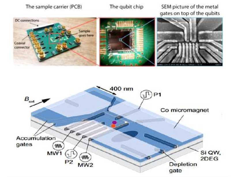
Fig. 3. Spin-Qubit Chip

There has been tremendous progress in quantum technologies in recent years and we soon expect to see quantum computing test beds with tens and hopefully soon hundreds or even thousands of qubits. As these test devices get larger, a full software stack for quantum computing is required in order to accelerate the development of quantum software and hardware, and to lift the programming of quantum computers from specifying individual quantum gates to describing quantum algorithms at higher levels of abstraction. The open source effort ProjectQ aims to improve the development of practical quantum computing in three key areas:

First, the development of new quantum algorithms is accelerated by allowing users to quickly implement them in a high-level language prior to using various software back-ends and analysis tools. For example, there is a resource counter, which provides performance information such as the number of gates and circuit depth of the compiled programs in order to determine the crossover point with classical algorithms.

Moreover, we provide efficient high-performance simulators and emulators. They are required to determine the resource estimates for quantum algorithms for which the success probability and/or the scaling with problem size are known asymptotically at best, e.g., the variational quantum eigensolver. Scalable quantum simulators allow us to run small quantum programs and extrapolate the performance in the absence of noise. Besides this, quantum simulators enable us to find bugs in quantum code in a very pragmatic way. While one may want to aim at proving a program to be correct, the complexity of a general quantum program can be even higher than of classical distributed programs for which we currently fail to verify even small subroutines such as, e.g., certain locks. As a consequence, we do not expect to be able to theoretically prove the correctness of every quantum program. Rather, we envision a combination of theoretic validation and pragmatic testing to be the approach of choice.

Second, the modular and extensible design of ProjectQ encourages the development of improved compilation, optimization, gate synthesis and layout modules by quantum computer scientists, since these individual components can easily be integrated into ProjectQ’s full stack framework, which provides tools for testing, debugging, and running quantum algorithms. For each component provided reference implementations which subsequently can be improved and easily benchmarked using our quantum programs such as Shor’s algorithm.

Finally, the back-ends to actual quantum hardware – either open cloud services like the IBM Quantum Experience or proprietary hardware – allow for the execution of quantum algorithms on changing quantum computer test beds and prototypes. Compiling high-level quantum algorithms to quantum hardware will facilitate hardware-software co-design by giving feedback on the performance of algorithms: theorists can adapt their algorithms to perform better on quantum hardware and experimentalists can tune their next generation devices to better support common quantum algorithmic primitives.

It is proposed to use a device independent high-level language with an intuitive syntax and a modular compiler design. The quantum compiler then transforms the high-level language to hardware instructions, optimizing over all the different intermediate representations of the quantum program, as depicted in Fig. 4.

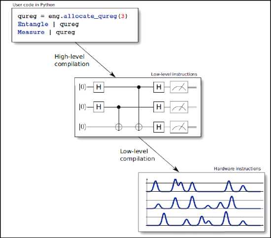
Fig. 4. High-level picture of what a compiler does

It transforms the high-level user code to gate sequences satisfying the constraints dictated by the target hardware (supported gate set, connectivity, ...) while optimizing the circuit. The resulting low-level instructions can then be translated into instructions for specific hardware, e.g., microwave pulse sequences, using the firmware provided by the different hardware platforms.

Programming quantum algorithms at a higher level of abstraction results in faster development thereof, while automatic compilation to low-level instruction sets allows users to compile their algorithms to any available back-end by merely changing one line of code. This includes not only the different hardware platforms, but also simulators, emulators, and resource estimators. Moreover, our modular compiler approach allows fast adaptation to new hardware specifications in order to support all qubit technologies currently being developed.

The high-level quantum language is implemented as a domain-specific language embedded in Python. To enable fast prototyping and future extensions, the compiler is also implemented in Python and makes use of the novel meta-instructions in order to produce more efficient code. Having the entire compiler implemented in Python is sufficient and preferred for current and near-term quantum test beds, as Python is widely used and allows for fast prototyping. If certain compiler components prove to be bottlenecks, they can be moved to a compiled language such as C++ using, e.g., pybind11. Thus, ProjectQ is ableto support both near-term testbeds and future large-scale quantum computers. As a back-end, ProjectQ integrates a quantum emulator, allowing to simulate quantum algorithms by taking classical shortcuts and hence obtaining speedups of several orders of magnitude. For the simulation at a low level, we include a new simulator which outperforms all other available simulators, including its predecessor. Furthermore, the compiler has been tested with actual hardware and one of our back-ends allows us to run quantum algorithms on the IBM Quantum Experience.

Noise is the central obstacle to building large-scale quantum computers. Quantum systems with sufficiently uncorrelated and weak noise could be used to solve computational problems that are intractable with current digital computers. There has been substantial progress towards engineering such systems. However, continued progress depends on the ability to characterize quantum noise reliably and efficiently with high precision. Figure 5 gives a complete description of the protocol for learning quantum noise.

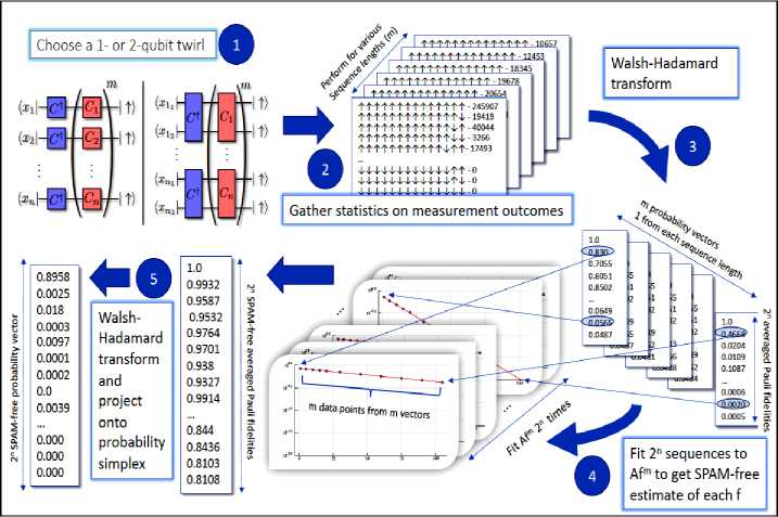
Fig. 5. An illustration of the protocol for characterizing the entire averaged probability vector for an n-qubit device [3].

It proceeds in five steps: First choose a number of long sequences of random quantum gates chosen independently from the single-qubit (or two-qubit) Clifford group, i.e., the group generated by the Hadamard, Phase, and (for two-qubits) CNOT gates on each individual qubit or qubit pair. Then estimate the resulting empirical probability distribution over the measurement outcomes and take a Walsh-Hadamard transform of the result. The resulting values will exhibit an exponential decay with respect to the sequence length parameter, m, so in step 4 it fit to such a model to learn the decay constants. Finally, it transforms back and project onto the probability simplex. This procedure provably converges to an estimate of the probability distribution of the average noise in the system, though the variant implemented here uses random gates chosen from the single-qubit Clifford group instead of the Pauli group. This leads to a simpler protocol, but one that additionally averages over the local basis information. The protocol presented in Fig. 5 reconstructs the full probability distribution with a number of experiments that scales polynomially in the number of qubits n, but requires computational resources that scale polynomially with the number of error rates to be estimated. The number of qubit error rates scales as 2n, so to make our protocol truly scalable, we need a method to estimate an efficient description of the noise that nonetheless captures the correlations in a transparent, systematic, and physically motivated way. The first experiments were run using the single-qubit protocol on the 14-qubit superconducting quantum architecture Melbourne, made available by IBM through the IQX online quantum computing environment. After completion of stage 4 of the protocol, it had reconstructed the entire averaged noise on the machine, returning all the qubit fidelities with multiplicative precision. The real utility of the protocol then comes from its unique ability to reconstruct the SPAM-free qubit error rates. This allows us to utilize the standard tools for analyzing probability distributions to understand the noise correlations in the device. Indeed, any functional of the reconstructed probability distribution can be computed from the data, such as the mutual information between pairs of qubits, the covariance matrix of the errors, or the correlation matrix (as in Fig. 6).

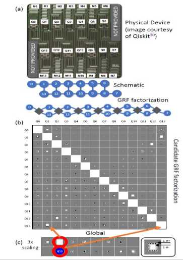
Fig. 6. Spatial layout of the qubits in the 14 qubit Melbourne architecture [3]

Edges in the schematic graph correspond to qubit pairs that can be coupled via a two-qubit gate. The factor graph below that is for a Gibbs random field (GRF) that model’s quantum noise via spatially local correlations in the device. Each diamond-shaped node is a factor that can describe arbitrary couplings among its constituent qubits. (b) The correlation matrix of the globally estimated distribution.

In particular, the covariance and correlation matrices can be computed unconditionally in polynomial time irrespective of any efficient GRF description by using the protocol. These tools provide invaluable diagnostic information about correlated errors that is difficult or impossible to obtain using prior art.

Learning models of quantum systems from experiments

An isolated system of interacting quantum particles is described by a Hamiltonian operator. Hamiltonian models underpin the study and analysis of physical and chemical processes throughout science and industry, so it is crucial they are faithful to the system they represent. However, formulating and testing Hamiltonian models of quantum systems from experimental data is difficult because it is impossible to directly observe which interactions the quantum system is subject to. Distilling models of quantum systems from experimental data in an intelligible form, without excessive over-fitting, is a core challenge with far-reaching implications. Great strides towards automating the discovery process have been made in learning classical dynamics. However, for quantum systems, these methodologies face new challenges, such as the inherent fragility of quantum states, the computational complexity of simulating quantum systems and the need to provide interpretable models for the underlying dynamics. Overcome these challenges here by introducing a new agent-based approach to Bayesian learning that we can successfully automate model learning for quantum systems. Several methods for the characterization of quantum systems with known models have been demonstrated. For example, when a parameterized Hamiltonian model H (x0) = Ho is known in advance, the parameters x that best describe the observed dynamics can be efficiently learned via Quantum Hamilto- nian Learning (QHL). However, these protocols cannot be used in cases with unknown Hamiltonian models: the description and modification of Hˆ are left to the user which is a major hurdle in automating the discovery process. Quantum Model Learning Agent (QMLA) to provide approximate, automated solutions to the inverse problem of inferring a Hamiltonian model from experimental data. The QMLA in numerical simulations tested and apply it to the experimental study of the open-system dynamics of an electron spin in a Nitrogen—Vacancy (NV) center in diamond. The QMLA is designed to represent models as a combination of independent terms which map directly to physical interactions. Therefore, the output of the procedure is easily interpretable, offering insight on the system under study, in particular by understanding its dominant interactions and their relative strengths. The overarching idea of the QMLA is that, to find an approximate model of a system of interest, a series of models are tested against experimental evidence gathered from the system. This is achieved by training individual models on the data, iteratively constructing new models of increasing complexity, and finally selecting the best model, i.e. of the models tested, the one which best replicates Hˆ . QMLA’s model search occurs across a Directed Acyclic Graph (DAG) with two components: structural (sDAG) and comparative (cDAG). Each node of the DAG represents a single candidate model, Hˆ . The DAG is composed layers µ , each containing a set of similar models, typically of the same Hilbert space dimension and/or number of parameters, Fig. 7a. For each Hˆ  in µ , QHL is used to find the best parameterization to approximate the system Hamiltonian Hˆ , yielding Hˆ→ Hˆ′ , Fig. 7b. The QHL update used for learning parameters is computed using the quantum likelihood estimation protocol depicted in Fig. 7e.

Classical likelihood evaluation can also be performed if the dimension of the Hilbert space is sufficiently small. Once all H ˆ ∈ µ are trained, µ is consolidated by systematically comparing models through Bayes Factors (BF) analysis, a measure for comparing the predictive power of different models that incorporates a form of Occam’s razor to penalize models with more degrees of freedom. Such comparisons are stored in the cDAG, Fig. 7c. The BF, denoted B penalizes models which impose higher structure, naturally limiting over– fitting.

Schematic of QHL used in b. A (quantum) simulator is used as a subroutine of a Bayesian inference protocol to learn the parameters of the considered Hamiltonian model. QHL chooses random probe states ψ and adaptive evolution times t , which are used both for the time evolution of the system and simulator. This retrieves the optimized parameterization x ′ . Spawn rules combine the previous layer champion, H ˆ ^µ , with the primitive’s library to determine models to constitute the next later υ .

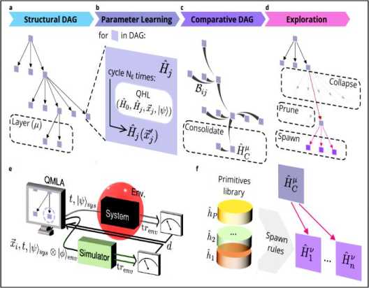
Fig. 7. a-d. Schematic representation of a single iteration of a QMLA instance [4].

Quantum Hamiltonian Learning (QHL) is the process of learning Hamiltonian parameters of an unknown quantum system by interfacing with a classical machine learning protocol, Bayesian inference (Fig. 8).

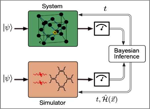
Fig. 8. Quantum Hamiltonian Learning: A quantum system (NV–center electron spin) is evolved, and a proposed Hamiltonian is run on a quantum simulator [5]

The true and simulated outputs are compared using Bayesian inference, leading to improved probability distributions over the parameter space. For example, the spin of an electron from a Nitrogen Vacancy center, which has been characterized, is known to have a Hamiltonian which depends on its Rabi frequency. In order to learn Hamiltonian parameters, it employs a form of approximate Bayesian Inference known as sequential Monte-Carlo Methods or particle filtering. This process iteratively improves the probability distribution over the parameter space. Quantum Hamiltonian Learning (QHL) designs experiments to run on the system of interest in order to maximize knowledge gained, and can invoke a trusted (quantum) simulator to test and iteratively improve parameterizations, resulting in trained x ′ (yielding H ˆ ′ ).

Often build abstract representations of physical systems that meaningfully encode information about the systems. The representations learnt by most current machine learning techniques react statistical structure present in the training data; however, these methods do not allow us to specify explicit and operationally meaningful requirements on the representation. A quantum fuzzy neural network architecture based on the notion that agents dealing with different aspects of a physical system should be able to communicate relevant information as efficiently as possible to one another. This produces representations that separate different parameters which are useful for making statements about the physical system in different experimental settings. Examples involving both classical and quantum physics. For instance, the architecture finds a compact representation of an arbitrary two-qubit system that separates local parameters from parameters describing quantum correlations. This method can be combined with reinforcement learning to enable representation learning within interactive scenarios where agents need to explore experimental settings to identify relevant variables.

The interpretability of QMLA’s outputs gives users a unique insight into the processes within their system of study. This can be helpful in diagnosing imperfect experiments and devices, aiding quantum engineers’ efforts towards reliable quantum technologies. Moreover, the potential to deepen understanding of physics provides a powerful application of noisy intermediate-scale quantum devices. The core of any QA is a set of unitary quantum operators or quantum gates. In practical representation, quantum gate is a unitary matrix with particular structure. The size of this matrix grows exponentially with the number of inputs, making it impossible to simulate QAs with more than 30 – 35 inputs on classical computer with von Neumann architecture. Background of quantum computing is matrix calculus.

In the three years since the original publication, the approach has been significantly improved. In one extension, the authors show how the usage of deep neural networks can lead to a speedup in finding useful output state. The idea is to train a neural network to classify the photon number distribution of a given state into one out of six categories (which involves cat states, squeezed cat states, cubic phases and others). The network helps to guide the search in the right direction, and only later, the computational expensive fitness functions are evaluated within the genetic algorithm. Thereby, several useful quantum states have been discovered. By improving both the numerical simulation and refining the search algorithm, quantum metrology, called Ada Quantum are able to improve the speed by another factor of five over their own best result.

Furthermore, they show higher noise and photon loss tolerance, which is essential in real experimental situations, see Fig. 9A, B, C, D.

Fig. 9(A). Outline of variational hybrid quantum-classical algorithm, in which we optimize over gate structures and continuous gate parameters in order to perform QAQC for a given input unitary U.

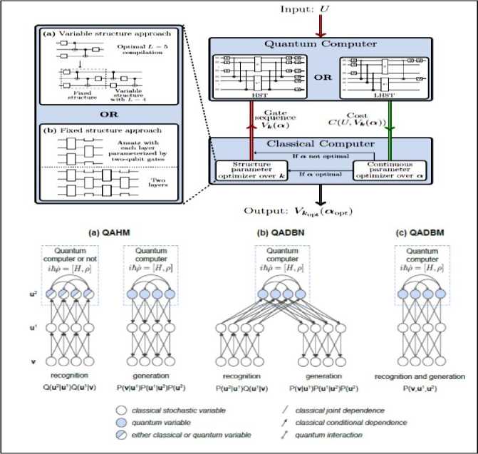
Fig. 9(B). Deep architectures for quantum-assisted generative modeling: (a) quantum-assisted Helmholtz machine (QAHM); (b) quantum-assisted deep belief network (QADBN); and (c) quantum-assisted deep Boltzmann machine (QADBM).

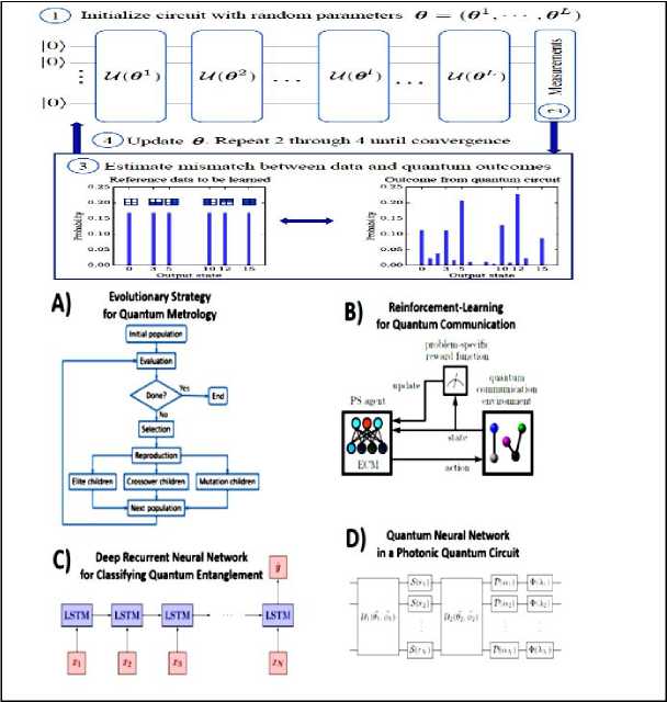
Fig. 9(C). Class of algorithms for computer-inspired quantum experiments with various optimization and machine learning techniques

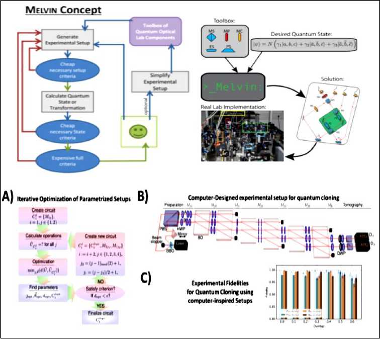
Fig. 9(D). Concept of the Class-III algorithm for computer inspired experiments, MELVIN [5].

In the quest for designing new quantum experiments, it faces two challenges: First, quantum phenomena are unintuitive. Second, the number of possible configurations of quantum experiments explodes combinatorially.

On Fig. 9 (C) a genetic algorithm for designing novel methods in quantum metrology. An initial, random population undergoes an evolutionary process. The individual setups, which form the population, are selected according to their fitness. The best ones are mutated and form the next generation. B) The concept of a reinforcement learning algorithm for designing quantum communication schemes. An agent performs actions in an environment (changing quantum communication scheme), which changes the state of the environment. The agent receives a reward according to the quality of the action. C) A deep recurrent neural network, based on long-short-term (LSTM) cells, receives optical elements in a sequence ( xi ), and learns to predict quantum entanglement properties of the setups y ˆ . In that way, the time-consuming objective function in a design process is approximated by a fast-neural network, which has the potential to speed up the search for new quantum entanglement experiments significantly. D) A photonic quantum circuit can be parametrized continuously, thus gradient-based optimization techniques are possible. The circuits topology here follows the quantum neural network Ansatz, which consists of unitaries U i , squeezing S , displacement D and non-Gaussian gates Φ. Data-driven quantum circuit learning. The training data is interpreted as representative of an unknown probability distribution. The generative task is to model such a distribution. Learning consists of updating the parameters 6 of a quantum circuit Born machine (QCBM) to minimize the mismatch between the data and the measurement outcomes.

As example, in accelerator physics, computer-inspired and computer-optimized designs have a long tradition, from which we mention a few interesting recent examples. Genetic algorithms augmented with machine learning techniques have been used to optimize the magnetic confinement configurations of National Synchrotron Light Source II (NSLS-II) Storage Ring (Brookhaven National Laboratory, New York, USA). The goal was to maximize the dynamic aperture, a complex multi-objective function that involves, among others the beam lifetime and energy acceptance and several high-quality solutions have been experimentally tested. If these promising proposals are indeed feasible experimentally, and yield the predicted phase measurement precision, they could become prime examples in experimental quantum metrology research.

Time-optimal Control of Qubit

To visually understand a qubit, we can understand it as a Bloch Sphere. This sphere shows the probabilities (a and 6) as being the determinate factors for the qubit and provides 3 degrees of freedom (originally 4 degrees of freedom but 1 is eliminated by the normalization constraint via the Born Rule). The twodimensional Bloch Sphere visualization and feature map is shown below. All of these transformations can also be visually recognized as shifts on the axis of a Bloch Sphere. For example, we can see the Pauli-X gate transformation mapped to the Bloch Sphere Fig. 10A.

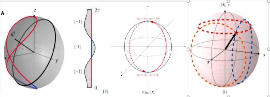
Fig. 10A. Quantum Registers: Bloch sphere with Bloch vector for the qubit state | ^ = — 10)

1 + i

The precession induced by a Hamiltonian proportional to a_x , Г and < r _z is indicated by the orange, blue and red circles, respectively. Results based on two experiments, commonly referred to as 'T 2 Ramsey'

and 'T 2 Echo'. Beginning with the Ramsey experiment, with a qubit initialized in the 0 state, the theoretical final state after two sequential Hadamard gates ( A t = 0 ) should return the qubit back to the ground state. However, when time is introduced in between these two H gates, the qubit becomes susceptible to T 2 transverse relaxation. Illustrated in Fig. P10B, the dephasing component of T 2 relaxation can be represented as a "drifting" effect around the equatorial plane on the Bloch Sphere, whereby one continually loses knowledge of the exact position of the state over time.

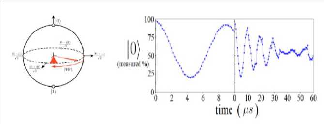
Fig. 10B. Bloch Sphere representation of the state of the qubit after being initialized by a Hadamard gate. The orange shaded areas in the equatorial plane represent the growing uncertainty in the state of the qubit, reaching a fully decoherent state after enough time. Data collected running the T 2 Ramsey circuit for two different time scales, both on the same qubit [6].

Physically, this effect causes the second Hadamard gate to transform the qubit to a new final state based on the elapsed time, one which oscillates between 0 and 1 with the frequency of the drift

IV (t))

I o)+ ei⁰¹

. The quantum circuits for the experiment are shown below in Fig. 10C.

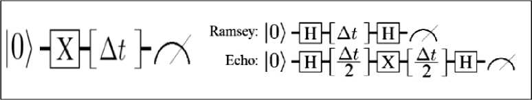
Fig. 10C: Quantum circuit for studying T1 coherence times (left). The qubit is excited into the 1 state via the X gate, followed by various amounts of time where the qubit may spontaneously undergo a T1 collapse. Quantum circuits for demonstrating the T2 nature of IBM's qubits (right). The difference between the two experiments can be seen in the extra X gate between the split At

In both experiments the qubit is initially brought into a 50 – 50 superposition state via a Hadamard gate, followed by various amounts of time A t , and finally a second Hadamard just before the measurement. During the time between Hadamard gates, the qubit is subject to both spontaneous energy relaxation ( T 1 ) as well as dephasing, for a combined referred to as transverse relaxation.

Let us discuss the single-qubit Bloch sphere (or ball) of qubit-A after a partial trace over qubit-B. Once qubit-B is traced out, the quasi-state vector | V) is no longer a well-defined quantity. The partial trace over qubit-B maps the two-quit density matrix p^= VAb)VAB I to the reduced density matrix pA. Similarly

(see Fig. 10D), let us define the partial trace over qubit-B as a map on the quasi-density matrix pA, TrB : pA ^ pA;

TrB : pA =	1 + x 0	x l - bt ^	^ p A =	1 + x o	X | - x^t
	x , + bt к 1	1 - x 0 у		x , + x.t к 1    4	1 - x 0 у

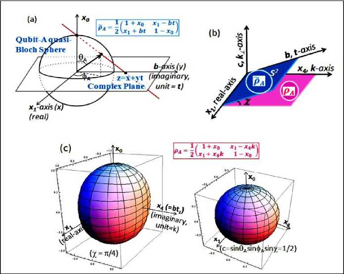
Fig. 10D. An illustration of the partial trace [7].

Three-unit spheres can represent the two-qubit pure states. The three spheres are named the base sphere, entanglement sphere and fiber sphere. The base sphere and the entanglement sphere represent both the reduced density matrix of one qubit (the base qubit) as well as the non-local entanglement measure, concurrence, while the fiber sphere represents the other qubit (the fiber qubit) geometrically under a local unitary operation. When the bipartite state becomes separable, the base sphere and the fiber sphere seamlessly become the single-qubit Bloch sphere of each qubit. Since either qubit may be chosen to be the base qubit, two sets of such spheres can fully represent the reduced density matrices of both qubits as well as the concurrence where the concurrence value is the same in the two sets.

The concurrence in this Bloch sphere is correctly related to the reduced density matrices. In particular, the entanglement (concurrence) and the imaginary part of coherence (off-diagonal element of the reduced density matrix) are related via an angle parameter and are represented together in the entanglement sphere. The fiber sphere, along with the phase factor, represents the fiber qubit geometrically in response to a local unitary operation, but otherwise it has no local information about the fiber qubit in an entangled state. In an entangled state, its main purpose seems to be to help the three Bloch spheres accurately represent the bipartite state. In a separable state, the fiber sphere is precisely the Bloch sphere of the fiber qubit. In the entangled states, the base sphere and the entanglement sphere (of the S 4 Hopf base) represent both the local information of the base qubit via its reduced density matrix and the non-local concurrence of the bipartite state. The fiber sphere represents the fiber qubit geometrically only, showing a simple rotation under a local unitary operation, otherwise it has no physical significance other than helping the three Bloch spheres accurately represent the bipartite state. In a separable state, the base sphere and the fiber sphere become exactly the single qubit Bloch sphere of each qubit. Figure 10E shows the entangling circuit with x - or y -rotation by angle n, R x,y ( 9 ), producing a linear superposition of the control-qubit, qubit- A .

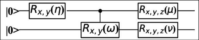
Fig. 10E. Two-qubit quantum circuit to generate partial entanglement between the two qubits with 0 <  concurrence <  1. The gates are the rotation operators. Concurrence = 0 for separable states and 1 for maximally entangled states (MES). For this circuit, concurrence = sin ( n ) sin ( ® / 2 ) and sin ( n ) is the degree of initial superposition of the control qubit

Note that the degree of superposition of |0^ and | |1^ states is sin ( n ) after this gate. The controlled x -or y -rotation, C - Rx y ( to ) , entangles the two qubits. The concurrence is given by sin ( n ) sin ( to /2 ) after these two gates.

Figure 10F shows the two sets of Bloch spheres after the Rx ( 60 ) ® I gate to induce the superposition in the control qubit- A and the C - Ry ( 70 ) gate to entangle the two qubits.

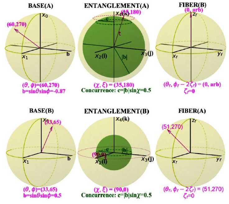
Fig. 10F. The two sets of Bloch spheres where qubit-A is the control qubit, after Rx ( 60 ) ® I

^ C - Ry ( 70 ) where the rotation angles are n = 60 degrees, to = 70 , and ц = v = 0 in the circuit of Fig.

10E. Top row: qubit-A is the base qubit. Bottom row: qubit-B is the base qubit [8].

If the base qubit local unitary operation changes the y- coordinate ( i.e. , b -changing operation), like the local x - and z -rotations, then all three spheres could change in response and the base sphere rotates as if it is in a coupled system of spheres. In presented Bloch sphere model, the local operations evolve the base and entanglement spheres while the fiber sphere has no physical significance as far as the base qubit is concerned. Therefore, the base and entanglement spheres maintain all local and non-local information for the base qubit and the bipartite state while leaving the physically inconsequential parts to the fiber sphere. Measuring the spin direction of the local, base qubit, the probability will always be cos² ( O /2 ) for spin up or the 0 state, whether the bipartite state is entangled or separable . Extend the coherent time and reduce the operation time with bounded energies are two common methods in general for this problem. To reduce the time of performing a quantum gate, the system needs to evolve as fast as possible, and the shortest time for performing a quantum operation or evolving a state to a target state, is now referred to as the quantum speed limit (QSL).

Quantum speed limit is a fundamental concept in quantum mechanics, which aims at finding the minimum time scale or the maximum dynamical speed for some fixed targets. In a large number of studies in this field, the construction of valid bounds for the evolution time is always the core mission, yet the physics behind it and some fundamental questions like which states can really fulfill the target, are ignored. Under- standing the physics behind the bounds is at least as important as constructing attainable bounds. Well-used method for the construction of QSL is the geometric approach, which utilizes the metrics and geodesic lines in some differential manifolds. One such example is the quantum Fisher information based on the symmetric logarithmic derivative, which is proportional to the Fubini-Study and Bures metrics for pure and mixed states. An inequality for the QSL A < J ^F (t)dT, where F(t) is the quantum Fisher information for the time t with A = arccos f the Bures angle, as well as the target angle, in this equation; f = Tr

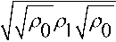
is the

fidelity between two quantum states p and p . In the case of a noncontrolled fixed Hamiltonian, the trajectory of evolution in state space is fixed for a fixed decoherence mode and strength, no matter the Hamiltonian is time-dependent or not, as shown in Fig. 11a.

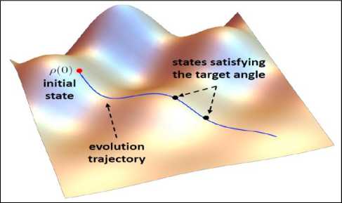
Fig. 11a. (Color online) Dynamical trajectory of a quantum state p ( 0 ) . Only one trajectory exists for a non-controlled fixed Hamiltonian with a fixed decoherence. The states satisfying the target angle are hence also fixed on this trajectory. Therefore, the QSL should not be a function of time in these cases

In principle, and perhaps intuitively, one might expect the complexity of many control systems to result in landscapes that possess large numbers of local optima. We shall, however, argue that a specific notion of complexity is favorable for control optimization rather than deleterious, to actually reduce the possibility of traps. Figures 11b and 11c illustrate some low-dimensional (two control parameters) examples. In practice, typically, many more control parameters than two are present and control landscapes cannot be directly visualized.

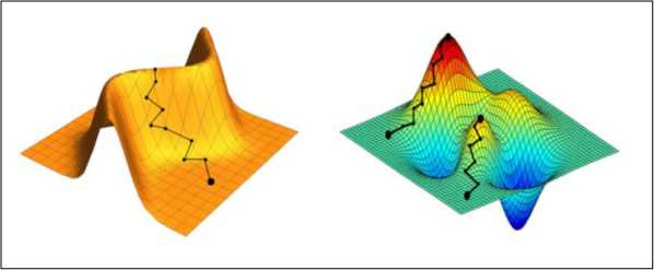
Fig. 11(b). A control landscape with a plateau (showing a one-dimensional critical manifold of global optima) but no with traps. Landscapes of this type, or even with additional saddle features, are highly favorable for finding optimal controls (c)

A local gradient search climbing the landscape reaching either dead-end sub-optimal traps or the desired true global optimum, depending on the starting point. Landscapes of this type, especially in high dimensions, are highly problematic for finding optimal controls

The critical point topology of a control landscape determines the behavior of local optimization algorithms, such as gradient ascent and even non-local stochastic algorithms could be greatly hindered by a rough, high-dimensional landscape. An understanding of the critical point topology, i.e. the set of controls where ∇F = 0, permits assessing the ease of finding optimal controls. Saddle points could exist on some landscapes, but they would only slow down a search rather than stop it from proceeding to full optimization. For an application of a gradient method in laboratory practice, in which the algorithm is applied to spectrally filtered and integrated second harmonic generation as well as excitation of atomic rubidium. In this work, monotonic convergence to maximum fidelity is seen within practical laboratory time scales. Work on assessing the experimental relevance of saddle points has also been undertaken in which their impact was found to be negligible, as theoretically expected. This is due to the fact that the solutions of states in a fixed differential equation is unique. Therefore, which states on the trajectory satisfy the target angle are actually fixed and determined by the trajectory itself, which is further determined by the parameters in the Hamiltonian and dissipative parameters, rather than the time t. Hence, the QSL should not be dependent on the time either. Most of the current theoretical tools cannot reveal this fact, especially for the time-dependent Hamiltonians. Thus, some new approaches are still in need in this field to reveal the true physics behind the QSL.

QSL in two-level systems (qubit)

The Hamiltonian of a two-level system in the energy basis is H = E_o | E_o) (E _o | + E | E) (Д |, here E _o, E_x are the energies and | E ₀}, | E j are corresponding eigenstates. Define | ^ ) as k z ) = | ^E 1) ( ^E 1| | E o) ( ^E 0 I ^, namely, the Pauli matrix in basis {| E _o},| E_x ^} . With the Pauli matrix, the Hamiltonian can be rewritten into

^H = 1 ( ^E o + ^E i )! + ( ^E i — ^E o 4

. The identity matrix commutes with any operator, hence it has nothing to do with the evolution. Then the Hamiltonian can be simplified into ^ (E1 - Eo) a_. In the Bloch represen- tation, this means the evolution of any state is the rotation of the corresponding Bloch vector about z-axis. A general vector in Bloch sphere can be expressed by r (n,a,ф) = n(sin a cos ф, sin a sin ф,cos a), where П g [0,1], a g [0, n], and ф g [0,2n]. For an initial state r (n, a, ф) , the evolved state is as follows r (n, a, ф) = n (sin a cos фcos (tot) - sin a sin фsin (tot), sin a cos фsin (tot) + sin a sin фcos (tot), cos a)

1             1                                _{1 P}             .            2 n      2 n

.

It can be seen in this equation that the period of the dynamics is T = — =------- to E - E_o

For any specific initial state r ( n , a , ^ ) , the set of all states on the evolution trajectory (denoted by <£*) is 8 = { r ( n , a , ф ) ^ g [ 0,2 n ] } . One may notice that the set of all target states for a specific initial state (denoted by T) here is a cone with the initial state as the axis. For any state r ( n , a , ф ) , the condition of r g S is that 8 and T have intersections.

l_f 9 ii                      -il

In the case that 8 = T = <  r I n , —, ф I1 Ф g [ 0,2 n ] >  for any specific n , as shown in the yellow cone in

Fig. 8(a). The coincidence between 8 and T means that all the states with n ^ 0 in 8 are in the set S , i.e.,

i 9 il                                         l

^ =' r \п^~ф Ф I |n g [0,1], ф g [0,2n] > g 5 . Furthermore, it is easy to see that for any specific state in this case, only one target state exists, i.e., the symmetrical state with respect to the initial state about z-axis. It requires half of the period to rotate the initial state to its symmetrical state, thus, the evolution time in this scenario is t = — = ———. Next, for the case that a < 9 /2 , all states within 8 (the blue cone in Fig. 12

(a)) fail the target 9 since the largest angle between the initial state and the evolved state is 2 a , which is smaller than 9 . This means any state satisfying a <  9 /2 is not in the set S .

Fig. 12. (Color online) Schematic of three scenarios for the calculation of the operational definition of QSL in a qubit system

• (a)    The case a < 6 /2 ( a is the angle between the initial state and the z -axis). When a < 6 /2 , there exists no target state fulfilling the angle 6 . When a = 6 /2, only one target state exists.

• (b)    The case a > 6 /2. For this case, two target states exist. (c) is the projection of initial and target states on xy -plane [9].

For the case that , 2 a >  6,8 (the blue cone in Fig. 12(b)) for any value of n ^ 0 shares two vectors with (the purple cone in Fig. 12(b)), which means any state in this scenario has two target states r and

,         X      г ,        6 г       ,      _ rtari on the evolution trajectory. Thus, ^2 = | r

(n, a,p) Ine [0,1], a > — ^ e [0,2n] ^ e S . Since the rota- tion is counter clockwise (looking against the z-axis), the evolution time to r is smaller than the one to rtar2. To calculate this evolution time, the angle between the projections of r = r (n, a,^) and rtarX on xy-plane (denoted as в) needs to know. From Fig. 12(c), it can be found that the length of the projection of r

( 6 ^

. Thus, the angle

is r sin a , and the length between these two projections is 2 r sin

(2 )

в = 2 arcsin

■  ( 6

sin sin a

2п в     2

, which indicates the evolution time is t =--=-------arcsin

E_x - E ₂ 2 n E - E₂

■  ( 6

sin

( 2

sin a

.

The minimum value of this evolution time is > —-— , which is attained at a = n /2 . Combing the ^E 1 - ^E 2

result obtained in the case of 2 a = 6 , one can finally obtain t >-------, and the set 5 = ^0 ST. The case

E i - E 2                     *    ²

with n-a can be analyzed in the same way.

A formalism based on Pontryagin's maximum principle is applied to determine the time-optimal protocol that drives a general initial state to a target state by a Hamiltonian with limited control, i.e., there is a single control field with bounded amplitude. The coupling between the bath and the qubit is modeled by a Lindblad master equation. Dissipation typically drives the system to the maximally mixed state, consequently there generally exists an optimal evolution time beyond which the decoherence prevents the system from getting closer to the target state. For some specific dissipation channel, however, the optimal control can keep the system from the maximum entropy state for infinitely long. The conditions under which this specific situation arises are discussed in detail. The numerical procedure to construct the time-optimal protocol is described. In particular, the formalism adopted here can efficiently evaluate the time-dependent singular control which turns out to be crucial in controlling either an isolated or a dissipative qubit. The following single-qubit control problem considered

H ( t ; u ) = a x + u ( t ) [ a _x + a z ] = Ho + u ( t ) Hd , with | u ( t )| - 1•

Parameter £ is a model parameter; the control u(t) is bounded; and a's are Pauli matrices defined as ax

, ^a y

0  - i i0

, ^a z

0  -1

. The initial and target states are chosen respectively as the

ground states of a + 2a _ and a — 2a_z , i- e.,

I Vin) =

1                1

7 io+475 l^{- 2} - 75.

1               1

71o - 475 l ² —75 _

Using the Bloch sphere representation where any general state can be represented by three angles one of

them is the overall phase) | у ( б, ф,ф )^ = е ^ф

^ cos ( ф /2 ) ^ _v е ^ф sin ( ф / 2 ) ^

,#

, in

~ 0.85 ^ , ^_и ~ 0.15 n (see, Fig. 6 b, d). For

the typical time-optimal control problem, one finds the optimal u* (t) that Vin) to Vj^ (UP to an arbi trary phase) in the shortest time and Hamiltonians of |u| = 1 are defined as Hx = Ho - Hd, HY = Ho + Hd ,

• i .e., H_x corresponds to u = -1 whereas Hy to u = +1. The dynamics of the system is governed by the

  Schrodinger's equation:

  
  

  i d t ^{V (} t

  
  

  = ^ H + u ( t ) H^ J | у ( t )^ The initial and target states are given above. To

  
  

make the final state у j-_m] as close to as possible, the terminal cost function can be chosen as

^C 1 ^ 1 t Jin ) ) = — jl f 'H t fin ))| . ^The results t in

= 0.42 n , % = 0,0.2 and 0.8 are given in Fig. 13.

The trajectories of ( # ( t ) , ф ( t ) ) can be visualized on a Bloch sphere [Fig. 9(b), (d), and (f)], from which clearly to see that the optimal trajectory and the singular arc overlap over a finite amount of time. Upon increasing £ , the singular arc tilts more (i.e., closer to the equator of the Bloch sphere) and the optimal control changes from XSY [Fig. 9 (a) and (c)] to YSY [Fig. 9 (e)].

It is interesting to consider the case of £ = 0 with unbounded | u ( t )|. As the singular arc is defined by ф = n /2, the trajectory under the time-optimal BSB control, that steers a general initial state I V _in } ^ ( ^ o, ф ₀ ) to a general target state | v^^.t ) ^- ( # 1 , ф 1 ) , goes through

^{( 6} Q , ^ф 0 ^)— 8^ ⁽ # 0 , ^П / 2 ^)— S ^⁽ # 1 , ^П / ^{2 )—} 8^ ⁽ # 1 , ^ф 1 ) .

B can be X or Y depending on the initial and final states. The times of the first and the last bang-control are both infinitesimal; the singular control takes the time # ₀ - # | /2.

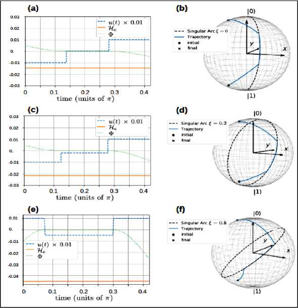
Fig. 13. The optimal control for the evolution time t_fin = 0.45 n .

• (a) and (b) for § = 0; (c) and (d) for § = 0.2. (e) and (f) for § = 0.8. (a), (c) and (e) show that all necessary conditions are satisfied. Dashed curves: scaled control; solid curves: c-Hamiltonian; dotted curves: switching function. (b), (d) and (f) show the corresponding singular arc (dashed curves) and the optimal trajectory (solid curves) on Bloch sphere. Note that the optimal control goes from XSY to YSY upon increasing § . [10]

Expressing | v_in } = i₀ 10) + i 11) = cos ( ^ / 2 ) 10^ + е ^ф sin ( ^ /2) |1) and,

| V t arg et } = t 0 | ⁰) ⁺ t 1 | ¹ = cos ( ^ 1 / ²) | ⁰) ⁺ ^ sin ( ³ / ² ) I 0

T min

(    ^    3 ,  •  ^ • ex)

= arccos ( ii_ot₀ + i_xt_x |).

= arccos cos — cos-- + sin — sin

I     2    2      2    2 )

This is “quantum speed limit”. Results of § = 0.8 will be shown to demonstrate the generality of some nonintuitive behavior found in systems with the o_x dissipation channel. Without dissipation, the minimum time to reach the target state is about 0.44 n for § = 0.8.

The Quantum Internet , i.e. a network enabling quantum communications among remote quantum nodes, has been recently proposed as the key strategy to significantly scale up the number of qubits. Such a quantum network may allow an exponential speed-up, of the quantum computing power with just a linear amount of physical resources, represented by the wired quantum processors. Indeed, by comparing the computing power achievable with quantum devices working independently vs. working as a unique quantum cluster, the gap comes out – as depicted in Fig. 14.

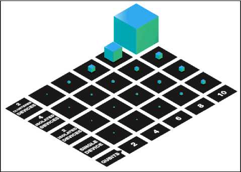
Fig. 14. Distributed quantum computing speed-up

The volume of cubes represents the ideal computational power, i.e., in absence of noise and errors. Interconnecting quantum processors via the Quantum Internet provides an exponential speed-up with respect to isolated devices.

Specifically, increasing the number of isolated devices lays to a linear speed-up, with a double growth in computational power by doubling the number of devices. Conversely, increasing the number of interconnected devices provides an exponential growth, with a significant advantage clearly visible with just two interconnected devices. As instance, a single 10-qubit processor can represent 210 states thanks to the superposition principle. But if we wire two processors, the resulting virtual device can represent up to 218 states, depending on the number of qubits devoted to quantum information sharing via the teleporting process. The distributed quantum computing from a communication engineering perspective, it is worthwhile to note that the availability of the Quantum Internet infrastructure scalable in the number of interconnected devices enables unparalleled capabilities not restricted to the distributed computing. Specifically, applications such as blind computing, secure communications and noiseless communications have already been theorized or even experimentally verified. Blind quantum computing refers to a server-client architecture where clients can send sensitive data to server, which elaborates inputs without knowing their values.

This functionality allows to achieve a twofold goal: preserving data confidentiality as well as solving tasks that are intractable for the client – that can be a classical computer – but tractable for the server, which implements the quantum paradigm.

The overall aim of classical distributed computing is to deal with hard computational problems by splitting out the computational tasks among several classical devices in order to lighten the loads on single devices. With the network infrastructure provided by the Quantum Internet, this paradigm can be extended to quantum computing as well: remote quantum devices can communicate and cooperate for solving computational tasks by adopting a distributed computing approach. Since an entirely new paradigm – characterized by unconventional phenomena ruled out by the quantum mechanics such as no cloning and entanglement is involved, a new infrastructure needs to be engineered.

The infographic in Fig. 15 is a stack depicting dependencies among a possible set of layers that together provide a distributed quantum computing ecosystem. For the sake of clarity, the attention is restricted to an infrastructure composed by two quantum devices, directly inter-connected. Nevertheless, the discussion in the following can be easily extended to more complex network architectures, provided that end-to-end routing and network functionalities are available. The lowest level provides the communication/network functionalities and consists of quantum devices interconnected through the Quantum Internet with both classical and quantum links. Thanks to underlying communication infrastructure, both local and remote qubit operations can be executed. Hence, from a computing perspective, the two lowest levels concur to build a virtual quantum processor with a number of qubits that scales with the number of quantum physical processors. This virtual processor is in turn controlled by the distributed compiler, which maps the quantum algorithm in a sequence of local and remote operations so that the available computing resources are optimized with respect to both the hardware and the network constraints.

At the very top we have the quantum algorithm, which is completely independent and unaware of the physical/logical constraints imposed by both the hardware and network configuration and particulars, thanks to the abstraction provided by the underlying levels.

Starting from bottom, in Fig. 15 we have the communication infrastructure underlying the Quantum Internet: spatially remote quantum devices able to communicate quantum information by means of a synergy of both classical and quantum communication technologies.

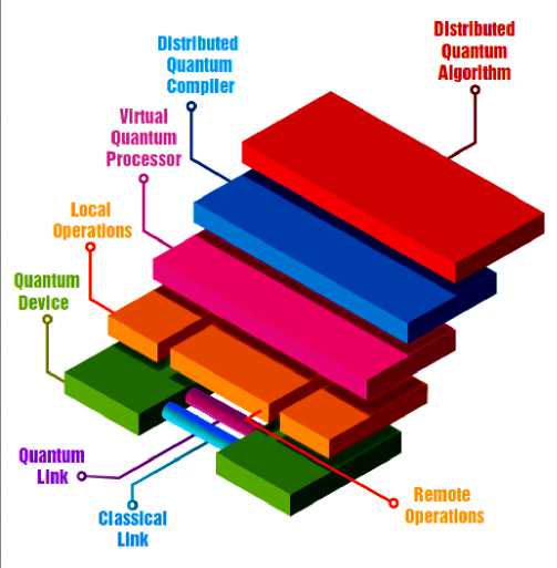
Fig, 15. A high-level system abstraction of a distributed quantum computing ecosystem

It is immediate to observe that only qubits linked by an edge can directly interact. Nevertheless, for an algorithm designer it is useful being able to define a circuit without restrictions on interactions. Indeed, a circuit quantum programming model can easily abstract from this restriction, resulting in a fully connected graph at the cost of an overhead due to indirect execution of the desired operation. For instance, let us consider to carry out a CNOT between the two non-adjacent qubits q 1 and q 3 of Fig. 16.

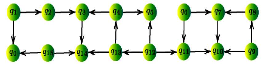
Fig. 16. Coupling map of the IBM QX3 architecture: the nodes represent the qubits while the edges represent the possibility to have interactions between two qubits, i.e., to implement the CNOT operation

As instance, a CNOT operation can be directly executed between qubits q 1 and q 2 but not between qubits q 1 and q 3 . By performing two swapping operations for each edge belonging to the shortest-path from node q 1 towards node q 3 , the overall result will be equivalent to a CNOT between q 1 and q 3 , keeping other states unchanged.

Figure 17 clarifies the process above.

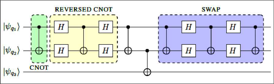
Fig. 17. A CNOT operation between non-adjacent qubits can be implemented through a sequence of swapping operations, with each swap consisting of three CNOT (with the in-between CNOT being reverse, i.e., with target and control qubits swapped) between adjacent qubits.

Note that the quantum state stored within qubit qi is denoted, by adopting the standard bra-ket notation for describing quantum states, as

ψ q_i

. Thus, the circuit performs a CNOT between q 1 and q 3 , leaving q 2

unaltered. The overhead induced by the swapping operations explains how important is the topological organization of device and the circuit design as well.

The quantum internet architecture requires both classical and quantum links. In this perspective, a distinction between matter and flying qubits – i.e., between qubits for information processing/storing and qubits for information transmission – must be made. As regards to the matter qubits, several candidate technologies are available, each one with its pros and cons. Conversely, as regards to the flying qubits, there exists a general consensus about the adoption of photons as qubit substrate. However, heterogeneity arises by considering the different physical channels the photons propagate through, ranging from free-space optical channels (either ground or satellite free space) to optical fibers. Thus, a transducer for matter-flying conversion is needed as depicted in Fig. 18.

ION TRIP

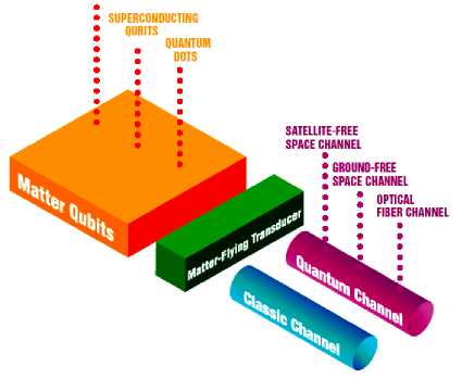
Fig. 18. Pictorial representation of a matter-flying transducer, which is needed to convert matter qubits – i.e., qubits for information processing/storing – into flying qubits – i.e., qubits for information transmission – and vice versa [11]

And communication models need to take into account such technological heterogeneity with the aim of providing a black box for upper protocol layers with one common logic.

Furthermore, quantum mechanics does not allow an unknown qubit to be copied or observed/measured. As a consequence, the communication techniques utilized to interconnect spatially remote quantum devices cannot be directly borrowed from classical communications. In this context, quantum teleportation is widely accepted as one of the most promising quantum communication technique between quantum nodes.

An important architecture of quantum computing is the computational model of adiabatic quantum computing (AQC) that started out as an approach to solving optimization problems. AQC permits quantum tunneling to explore low-cost solutions and ultimately yields a global minimum. It also exhibits convergence to the optimal or ground state with larger probability than simulated annealing. AQC devices intrinsically realize quantum annealing algorithms to solve combinatorial optimization problems giving birth to the paradigm of adiabatic quantum optimization (AQO). AQO is an elegant approach that helps escape local minima and overcomes barriers by tunneling through them rather than stochastically overcoming them as shown in Fig. 19a.

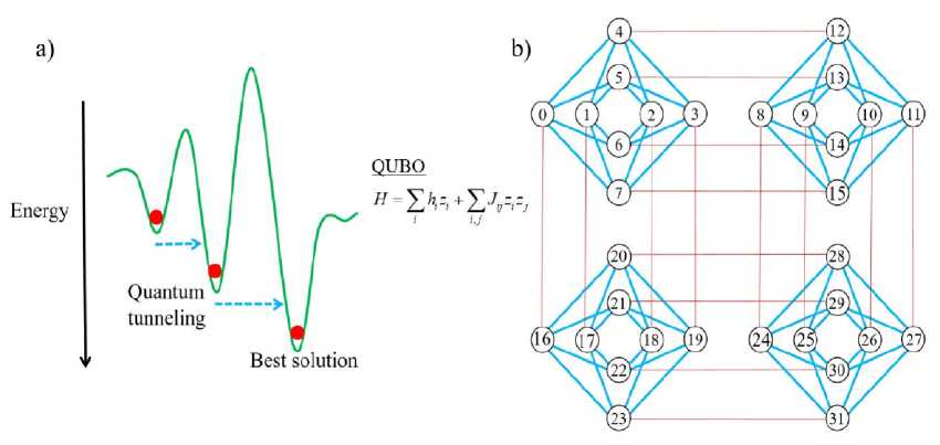
Fig. 19A. a) Adiabatic quantum optimization (AQO) and b) Chimera architecture of the D-wave processing unit

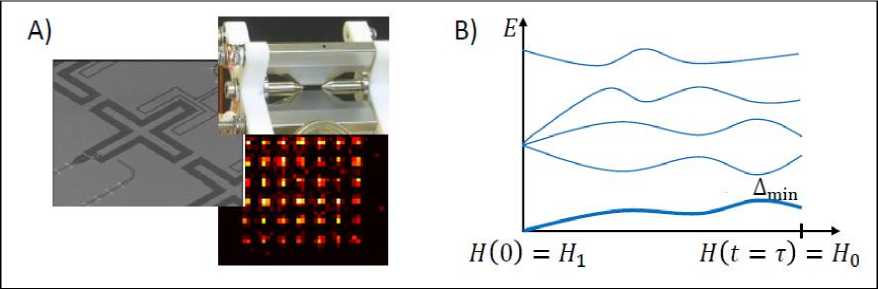
Fig. 19B. (A) Recent years have seen exciting developments on quantum-technology platforms (exemplified here by superconducting qubits, trapped ions, Rydberg atoms) These enable the implementation of quantum annealing protocols with the aim of solving hard optimization problems. (B) Sketch of time-dependent energy spectrum.

The solution to the optimization problem is encoded in the ground state of a problem Hamiltonian H0. It is reached at the end time τ of a slow sweep starting from the ground state of a Hamiltonian H 1 that is simple to prepare. If the sweep is sufficiently adiabatic (i.e., slow as compared to an inverse polynomial of the minimum gap Δ ), the system remains in the instantaneous eigenstate throughout (thick line). This article discusses experimental as well as theoretical prospects to boost the performance of such quantum annealers. Picture credits panel A (clockwise from left): MIT Lincoln Laboratory; Blatt group, University of Innsbruck; LCF, Instituted Optique, CNRS.D-Wave 2000Q and the Chimera graph.

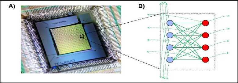
Fig. 19C. (A) Photograph of a D-Wave 2000Q Washington chip with 2048 qubits. From the web page of D-Wave Systems Inc. (B) Chimera graph unit cell and connectivity. Bullets indicate qubits within the unit cell and solid lines connections between them. Dashed arrows indicate connections to adjacent unit cells, which are arranged in a square-lattice pattern.

AQO can also be referred to as the class of procedures for solving optimization problems using a quantum computer. In AQC, the computation proceeds by moving from a low-energy eigenstate of the initial Hamiltonian to the ground state of the final Hamiltonian. A Hamiltonian mathematically describes the physical system in terms of its energies, and corresponds to the objective function of an optimization problem in the final Hamiltonian. The adiabatic optimization process evolves the quantum state towards a user-defined final problem Hamiltonian, while simultaneously reducing the influence of initial Hamiltonian in an adiabatic manner. Tunneling between various classical states or the eigenstates of the problem Hamiltonian is governed by the amplitude of the initial Hamiltonian. Decreasing this amplitude from a very large value to zero drives the system into the ground state of the problem Hamiltonian that corresponds to the optimal solution of the objective function.

In order to solve optimization problems with AQC, they need to be formulated as an Ising model or quadratic unconstrained binary optimization (QUBO) problems. Such QC devices that are designed to implement AQO are commercially made available by D-Wave systems. The quantum processing unit on D-Wave devices is represented as a lattice of qubits interconnected in a design known as Chimera graph. Figure P15b is a subgraph of the Chimera lattice pattern that is typical of the D-Wave systems and their operation. The objective function represented as an Ising model or a QUBO problem has to be mapped to the qubits and couplers of the Chimera lattice. Mapping of variables to the qubits requires a process called minor embedding. Embedding is an important step since the Chimera lattice is not fully connected. The adiabatic optimization process follows after the mapping of the objective function onto the physical quantum processing unit that searches for low-energy solutions of the corresponding problem Hamiltonian. The embedding and annealing schedule dictate the probability of recovering global optimal solutions.

The behavior of AQC systems in the presence of noise highly influences its performance and has been a subject of interest among researchers. Generic results for the Hamiltonian-based algorithm perturbed by particular forms of noise have also been reported. Adiabatic computation requires the gap between the excited states and the ground states to be not too small. Adiabatic evolution is particularly susceptible to noise if this gap is small. It has also been shown that under certain conditions, thermal interactions with environment can improve the performance of AQC. Apart from thermal fluctuations, several internal and external factors contribute to the noise in quantum systems. Qubits in such devices can be affected by the electronic control components and material impurities, which give rise to the external and internal sources of noise, respectively. In the context of optimization, noisy qubits deviate the state of the system from a global optimal solution to sub-optimal solution state. However, from a machine learning perspective, such noisy behavior and measurement uncertainty in quantum systems can be exploited to approximate sample distributions that could be used to model the distribution of data, as will be introduced in Quantum Generative Training.

Figure 20 summarizes the quantum generative training process that uses quantum sampling to find the maximum likelihood estimates of the corresponding model parameters.

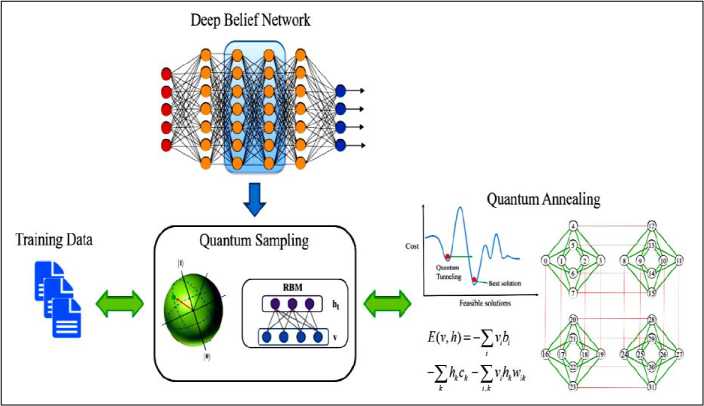
Fig. 20. Quantum generative training through quantum sampling [12].

With the approximate knowledge of the underlying Boltzmann distribution, the model expectations are computed by drawing several samples corresponding to the RBM energy function by quantum sampling.

With the increasing importance of water-energy-food nexus, challenges that account for its multiple scales, appropriate system boundaries, modelling the decision making and conflicting objectives along with uncertainties must be considered. Although a higher level of detail provides more thorough details, the associated modelling and computational challenges increase. Custom algorithms for a specific problem class can sometimes outperform the best available classical solvers, but a generic solution approach is much more desirable. While solving large instances of complex problems with deterministic technique is intractable, approximate algorithms should be considered. Quantum computers realize such approximate algorithms intrinsically.

Important large-scale problems of practical relevance can consist of thousands of variables, and constraints which due to their complex combinatorial nature may require days or even weeks to converge to an optimal solution. Design of shale-gas supply chain network covering more than 10,000 km ² area requires optimizing a mixed-integer linear problem with 51,133 variables and 51,880 constraints. State-of-the-art classical CPU-based solver takes more than 15 hours to compute a solution with the desired optimality gap. Another such example of an integrated optimization framework for energy supply chain involves optimization of a quadratic constrained mixed-integer problem with 8,321 total variables and 7,247 constraints. Solving this problem by a classical CPU-based solver requires 15.6 hours of computation time.

A quantum circuit comprises of quantum gates manipulating qubits to perform calculations. Analogous to logic gates in classical digital circuits, quantum gates are the building blocks of quantum circuits. In this model, quantum gate operations are applied one by one to the state of the system, thus evolving it towards a desired solution of the problem. Gate model of quantum computation is an alternate term used for this model. In the quantum circuit, the tasks of preparing a specific input, applying a set of gate operations and measuring the state of qubits in the computational basis is carried out sequentially.

Quantum algorithms play a vital role in implementing the power of quantum hardware. Approximate solutions for combinatorial optimization problems can be produced by Quantum Approximate Optimization Algorithm (QAOA). In the field of chemistry and optimization, a classical-quantum hybrid algorithm called Variational Quantum Eigensolver (VQE) has shown exceptional performance in terms of speed and resource utilization. Generating a trial state and estimating its energy is performed on a quantum computer with the energy being optimized on classical computer.

Recent developments in the field of quantum computation offer a way forward for determining efficient solutions of many instances of large eigenvalue problems that are classically intractable. Quantum approaches to finding eigenvalues have previously relied on the quantum phase estimation (QPE) algorithm. The QPE algorithm offers an exponential speedup over classical methods and requires a number of quantum operations O(p-1) to obtain an estimate with precision p. In the standard formulation of QPE, one assumes the eigenvector ψ of a Hermitian operator 7Y is given as input and the problem is to determine the corre- sponding eigenvalue X . The time the quantum computer must remain coherent is determined by the necessity of O (p 1) successive applications of e"mt, each of which can require on the order of millions or billions of quantum gates for practical applications, as compared to the tens to hundreds of gates achievable in the short term.

Here we introduce an alternative to QPE that significantly reduces the requirements for coherent evolution. A reconfigurable quantum processing unit (QPU) developed, which efficiently calculates the expectation value of a Hamiltonian ( ), providing an exponential speedup over exact diagonalization, the only known exact solution to the problem on a traditional computer. The QPU has been experimentally implemented using integrated photonics technology with a spontaneous parametric down conversion single photon source and combined with an optimization algorithm run on a classical processing unit (CPU), which varia-tionally computes the eigenvalues and eigenvectors of . By using a variational algorithm, this approach reduces the requirement for coherent evolution of the quantum state, making more efficient use of quantum resources, and may offer an alternative route to practical quantum-enhanced computation. In essence, we dramatically reduce the coherence time requirement while maintaining an exponential advantage over the classical case, by adding a polynomial number of repetitions with respect to QPE.

Example: Quantum variational eigensolver

The procedure outlined above replaces the long coherent evolution required by QPE by many short coherent evolutions. In both QPE and QEE we require a good approximation to the ground-state wavefunction to compute the ground-state eigenvalue, and we now consider this problem. Previous approaches have proposed to prepare ground states by adiabatic evolution, or by the quantum Metropolis algorithm. Unfortunately, both of these require long coherent evolution. The quantum variational eigensolver (QVE) algorithm is a variational method to prepare the eigenstate and, by exploiting QEE, requires short coherent evolution. QEE and QVE and their relationship are shown in Fig. 21.

Quantum variational eigensolver

Quantum expectation estimation

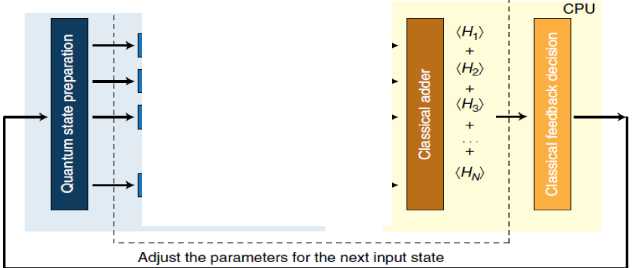
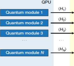
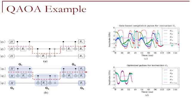
Fig. 21. Architecture of the quantum-variational eigensolver

In QEE, quantum states that have been previously prepared are fed into the quantum modules, which compute \ , where 7^ is any given term in the sum defining "И . The results are passed to the CPU, which computes /HS. In the quantum variational eigensolver, the classical minimization algorithm, run on the CPU, takes (^ \ and determines the new state parameters, which are then fed back to the QPU.

It is well known that the eigenvalue problem for an observable represented by an operator Tt can be restated as a variational problem on the Rayleigh–Ritz quotient, such that the eigenvector ψ ^ corresponding ψψ )

to the lowest eigenvalue is the ψ / that minimizes           . By varying the experimental parameters in

ψψ )

the preparation of ψ and computing the Rayleigh–Ritz quotient using QEE as a subroutine in a classical minimization, one may prepare unknown eigenvectors. At the termination of the algorithm, a simple prescription for the reconstruction of the eigenvector is stored in the final set of experimental parameters that define ψ .

If a quantum state is characterized by an exponentially large number of parameters, it cannot be prepared with a polynomial number of operations. The set of efficiently preparable states are therefore characterized by polynomially many parameters, and we choose a particular set of ansatz states of this type. Under these conditions, a classical search algorithm on the experimental parameters that define ψ needs only explore a polynomial number of dimensions—a requirement for the search to be efficient. One example of a quantum state parameterized by a polynomial number of parameters for which there is no known efficient classical implementation is the unitary coupled cluster ansatz.

The QPU have implemented using integrated quantum photonics technology; device, shown schematically in Fig. 22, is a reconfigurable waveguide chip that can prepare and measure arbitrary two-bit pure states using several single-qubit rotations and one two-qubit entangling gate.

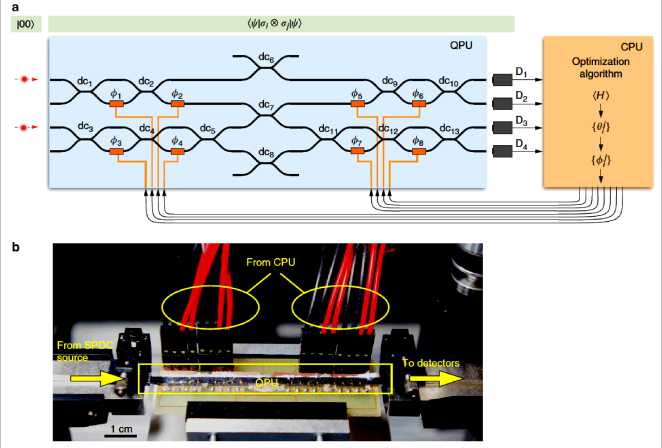
Fig. 22. Experimental implementation of the scheme.

• (a) Quantum-state preparation and measurement of the expectation values ψ σ _i ⊗ σ _j ψ are performed using a quantum photonic chip. Photon pairs, generated using spontaneous parametric down conversion, are injected into the waveguides encoding the 00 state. The state ψ is prepared using thermal phase shifters φ (orange rectangles) and one CNOT gate and measured using photon detectors. dc {1–4,9–13} ( dc 5–7 ) are 50% (30%) reflectivity directional couplers. Coincidence count rates from the detectors D 1 –4 are passed to the CPU running the optimization algorithm. This computes the set of parameters for the next state and writes them to the quantum device. (b) A photograph of the QPU.

The state is path-encoded using photon pairs generated via a spontaneous parametric down conversion process.

Figure 23a demonstrates the convergence of the average energy, while Fig. 23b demonstrates the con- vergence of the overlap Wj WG) of the current state Wj) with the target state W

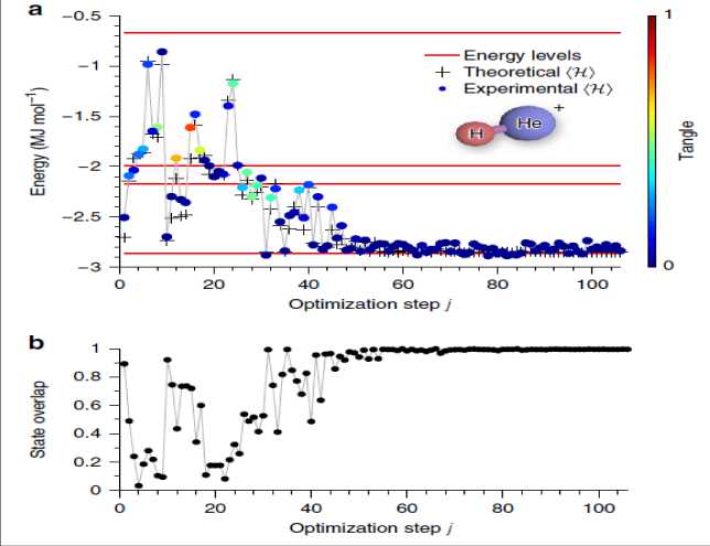
Fig. 23. Finding the ground state of He–H+ for a specific molecular separation R = 90 pm.

(a) Experimentally computed energy (colored dots) as a function of the optimization step j. The color represents the tangle (degree of entanglement) of the physical state, estimated directly from the state parameters {^j}. The red lines indicate the energy levels of ?f(R). The optimization algorithm clearly converges to the ground state of the molecule, which has small but non-zero tangle. The crosses show the energy calculated at each experimental step, assuming an ideal quantum device. (b) Overlap Wj |wG) between the experimentally computed state |wj) at each optimization step j and the theoretical ground state of H|wG) [13].

The color of each entry in Fig. 23a represents the tangle (absolute concurrence squared) of the state at that step of the algorithm. It is known that the volume of separable states is doubly exponentially small with respect to the rest of state space. Thus, the ability to traverse non-separable state space increases the number of paths by which the algorithm can converge and will be a requirement for future large-scale implementations. Moreover, it is clear that the ability to produce entangled states is a necessity for the accurate description of general quantum systems where eigenstates may be nonseparable—for example, the ground state of the He–H ⁺ Hamiltonian has small but not negligible tangle.

Error bars are smaller than the data points. The corresponding theoretical curve shows the numerically exact energy derived from a full configuration interaction calculation of the molecular system in the same basis. More than 96% of the experimental data are within chemical accuracy with respect to the theoretical values. At the conclusion of the optimization, we retain full knowledge of the experimental parameters, which can be used for efficient reconstruction of the state | W in the event that additional physical or chemical properties are required.

However, practical applications of the gate model quantum computer are limited. Few problems like integer factorization and solving linear system of equations show exponential speedup, while for other problems gate model quantum computers are not known to be faster than CPU/GPU-based classical computers.

The qubits in this model are susceptible to de-coherence, meaning their quantum states are destroyed by interactions with the environment. A universal quantum computer can be realized after overcoming these setbacks and joining forces with classical computing. Tech giants in the field of computation like IBM have already launched a cloud based commercial version of a gate model quantum computer, and is working towards building an universal quantum computer. IBM Q is an initiative to develop scalable quantum systems with a long term goal to realize an universal quantum computing system. Their devices can be accessed through an open-source quantum computing framework called Qiskit. Qiskit has three primary components, Terra, Aqua, and Aer, and they provide for composing quantum programs at circuit-level, tools and libraries for building quantum applications, and a high-performance simulator for quantum circuits, respectively.

A code sample written in Python programming language is shown in Fig. 24a where a quadratic assignment problem instance is solved using a quantum algorithm.

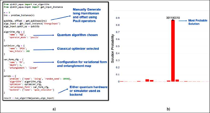
Fig. 24. a) Python code sample showing the use of Qiskit to solve a problem instance, and b) Histogram representing likelihood of possible solutions

In case of custom user defined problems, the Ising Hamiltonian needs to be manually generated. Exploring the open-source codebase for the various Ising translators should serve this purpose. The VQE quantum algorithm is chosen here among all those available in the Aqua library. A classical optimization technique and a variational method to calculate approximate wave functions along with an entangler map which specifies the entanglement of qubits are selected, depending on their specific properties and relevance to the ultimate goal. Finally, the quantum algorithm can be run on a Qasm simulator or on IBM Q devices remotely via cloud.

D-Wave systems use quantum annealing process to search for solutions to a problem. The D-Wave 2000Q system contains a quantum processing unit (QPU) with 2048 qubits. To solve hard problems with quantum computer, D-Wave provides a set of open-source Python tools called Ocean software development kit. A problem along with the user specified parameters is submitted to the QPU, and problem solutions corresponding to the optimal configuration of qubits are returned over the network. A sample code using the Ocean software libraries to solve the quadratic assignment problem instance and likelihood of best feasible solutions is shown in Fig. 25, where the ‘linear’ and ‘quadratic’ terms are user defined.

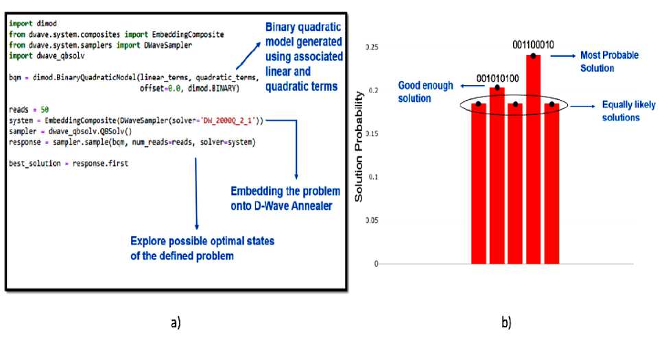
Fig. 25. a) Python code sample showing use of Ocean software libraries to solve a problem instance, and b) Histogram representing likelihood of possible feasible solutions [12]

Dimod is an utility that generates the binary quadratic model using both linear and quadratic terms provided. Embedding of the problem by mapping it to physical qubits on the annealer is an important step here. Qbsolv is a decomposing solver which finds the minimum of a large QUBO by partitioning it into smaller sub-problems. This solver can be configured to solve the QUBO problem instance by a meta-heuristic algorithm, Tabu Search, on a CPU-based classical computer or by quantum algorithm on D-Wave’s quantum system.

A crucial milestone in the field of quantum simulation and computation is to demonstrate that a quantum device can compute certain tasks that are impossible to reproduce by a classical computer with any reasonable resources. Such a demonstration is referred to as quantum supremacy. One of the most important questions is to identify setups that exhibit quantum supremacy and can be implemented with current quantum technology. The two standard candidates are boson sampling and random quantum circuits. Thus, quantum supremacy can be obtained in generic periodically-driven quantum many-body systems. Quantum computational supremacy is the ability of quantum devices to compute certain tasks that cannot be efficiently computed on a classical computer.

Early proposals for realizing quantum supremacy include boson sampling and random quantum circuits. In both cases, the computational hardness stems from the inability of a classical computer to efficiently approximate output probabilities of a complex quantum evolution. Experimental efforts towards achieving quantum supremacy include optical networks for boson sampling and superconducting circuits for random circuits. Signatures of quantum supremacy have been observed recently with 53 superconducting qubits. Generic isolated periodically-driven interacting quantum systems, when thermalized, cannot be efficiently simulated on a classical computer. These constitute a large class of quantum simulators that are currently available. The Eigenstate Thermalization Hypothesis (ETH) states that isolated many-body quantum systems thermalize by their own dynamics after a long enough time, regardless of their initial state. as long as ETH holds, periodically driven interacting quantum systems cannot be efficiently simulated on a classical computer in the worst-case scenario. The results open up possibilities to realize quantum supremacy in a wide range of experimental platforms.

The ETH states that isolated many-body quantum systems thermalize by their own dynamics after a long enough time, regardless of their initial state. But not only thermalization still occurs, but that for low-frequency driving, the associated temperature becomes infinite. In this limit, the Floquet operator Uˆ is described by a random matrix drawn from the Circular Orthogonal Ensemble (COE). This randomness is the particular ingredient responsible for the hardness in calculating the output probability, as there are exponentially many random Feynman trajectories that are equally important. By definition, a COE unitary evolution can be written as Uˆ = Uˆ T Uˆ . where Uˆ is a random matrix drawn from the Circular Unitary Ensemble (CUE). The latter is the ensemble of Haar-random matrices. random quantum circuits consisting of n + 1layers of gates and log2 N qubits, as shown in Fig. 26 (a).

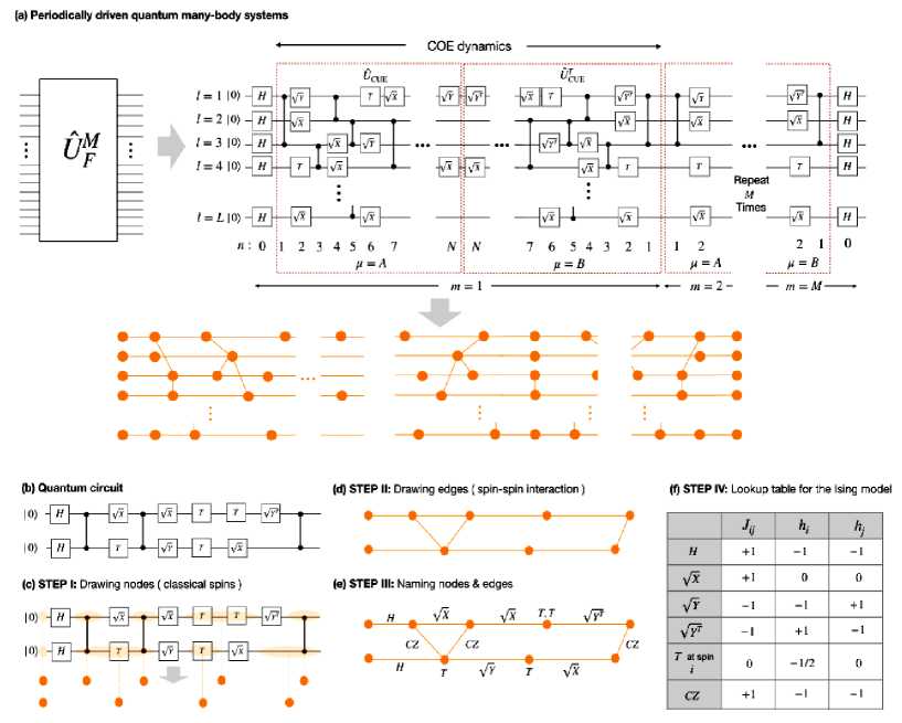
Fig. 26. Mapping driven many-body dynamics to complex Ising lattices

• (a) An example of a random circuit that generates COE dynamics and its conversion to the Ising model. (b) An example of a simple random quantum circuit, illustrating the mapping to the classical Ising model. STEP I to STEP III in the diagrammatic procedure are shown in (b) – (d), respectively. (e) Lookup table for the contribution of each gate to the local fields and the interaction in the Ising lattice.

Figure 27 shows the l1-norm distance between Pr(p) and the Porter-Thomas distribution at different m for the Ising and the Bose-Hubbard models.

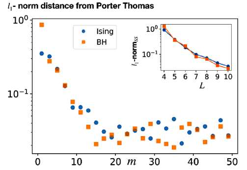
Fig. 27. The l1-norm distance between the output distribution from different quantum systems and the Porter-Thomas distribution at different m

The results from the Ising chain, the Bose-Hubbard chain, and random quantum circuits are labeled as crosses, squares, and circles, respectively [13].

It can be seen that, in all cases, the system reaches the Porter-Thomas distribution after multiple driving cycles. The l1-norm distance in the long-time limit is decaying towards zero as the size of the system increased. Therefore, the anticoncentration condition is satisfied.

New algorithms and new algorithmic paradigms (such as adiabatic computing which is the quantum counterpart of simulated annealing) have been discovered. We can explore several aspects adiabatic quantum computational model and use a way that directly maps any arbitrary circuit in the standard quantum computing models to an adiabatic algorithm of the same depth.

A quantum algorithm consists of a sequence of operations and measurements applied to a quantum processor. To date, the instruction set which defines this sequence has been provided by a classical computer and passed via control hardware to the quantum processor. Here, we demonstrate the first experimental realization of a quantum instruction set, in which a fixed sequence of classically defined gates performs an operation that is fully determined only by a quantum input to the fixed sequence.

Programmable computation, whether classical or quantum, consists of two fundamental components: an instruction set, and a machine to execute those instructions. For classical computation, there is no intrinsic distinction between these components - the same physical instrument may be used both to generate and execute the instructions (Fig. 28A). To date, the same has not been true for experimental demonstrations of quantum computing, whether in gate-based systems, quantum annealing, or one-way quantum computing. In conventional quantum computing applications, shown schematically in Fig. 28B, the instructions are programmed using classical resources and then delivered via hardware to a quantum processor that executes the instructions. In other words, the parity between instruction set and the processor executing the instructions is broken: one is fully classical, the other quantum.

An implementation of quantum instructions demonstrated, in which a quantum state provides on-the fly programming to a quantum computer (Fig. 28C). In this approach, a fixed sequence of classically-defined gates form the scaffolding for a variable operation on a target system с ; an auxiliary quantum state with density matrix completes the encoding of the instructions. This hybrid approach to quantum programming partially restores the parity between the instructions and the processor in a quantum computer.

Quantum instructions have a variety of applications, including executing private quantum functions and quantum simulation. Quantum instructions are central to an efficient implementation of quantum emulation, which enables the implementation of an unknown unitary U with a finite set of known input-output relations { ^ }— - —>{ p _out} . Quantum emulation consumes fewer copies of the instruction qubits than would be sufficient for tomographic reconstruction, enabling the application of U to an arbitrary state without compromising the privacy of U itself. A quantum instruction set has also been theoretically proven to provide quantum speedups in quantum semi-definite programming. Additionally, if a Hamiltonian is encoded in the instruction state, quantum instructions enable sample-optimal Hamiltonian simulation.

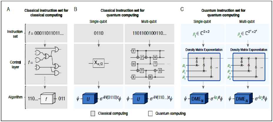
Fig. 28. (A) Schematic representation of classical computing

Instructions are expressed by a classical function f defined by a bitstring ‘00011...’, and is then executed on a dataset 110.... (B) Schematic representation of conventional quantum computing. The instruction set encoding a quantum circuit is generated using classical resources. A control layer generates the corresponding gate sequence, which is sent to the quantum hardware and implements the operation U = exp (-iH (0110) t) . Here H (0110) is the Hamiltonian with parameters given by the bitstring 0110. (C) Quantum instruction set using the density matrix exponentiation (DME) algorithm. A single-qubit instruction (p) is used to implement the operator DME^ (p,N,9)» exp(-ip9) using a sequence of N partial SWAP operations, each supplied with a new copy of (p ). A multi-qubit program using quantum instructions shares the same structure of the classical gates.

A quantum instruction set can be implemented efficiently using an approach called density matrix exponentiation (DME). DME consumes N copies of the quantum instruction density matrix p , and approximately performs the unitary gate exp ( - i p9 ) , where 9 is an arbitrary angle. It has been shown that DME asymptotically outperforms any tomographic strategy to implement exp ( - i p9 ) . Without access to a quantum instruction set, implementing exp ( - i p9 ) necessitates a full tomographic construction of p . This in turn requires O ( d 2 / £ 2 ) copies of p , where d is the dimension of the instruction system and £ is the desired precision. DME as implemented with quantum instructions requires only O ( 9 ² / £ ) copies, resulting in an exponential reduction in resource requirements. This advantage makes DME a powerful platform to implement quantum operations based on quantum states, avoiding the need for classical learning of p .

In Fig. 29, we implement a variant of DMEN in which one qubit serves as the target upon which the algorithm acts, and the other provides all N copies of the quantum instruction. This resource-efficient protocol, which we denote DME, trades a moderate increase in algorithmic error for a significant reduction in the required number of qubits.

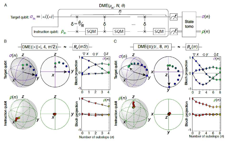
Fig. 29. (A) Two-qubit DME implementation using the SQM gate to approximately reinitialize the instruction qubit to p

The substep parameter n is stepped from 0 to N . We perform n rounds of § SWAP + SQM, measure the two-qubit density matrix, and trace over each subsystem to extract the individual density matrices с ( n ) and p ( n ) . (B) Substeps of DME(| +)(+| ,4, п /2), corresponding to R_x ( п 1 2 ) on the target qubit at the final step ( n = N) . Black lines are guides to the eye. (C) Substeps of DME(| |+)(+| ,8, п ), corresponding to R x ( п ) the target qubit at n = N . [14]

This approach relies on approximately re-initializing the instruction qubit after each § SWAP, without the need for active feedback, using a novel probabilistic operation which we call the simulated quantum measurement (SQM).

Many quantum algorithms developed for the so-called oracle model in which the input is give as an oracle so that the only knowledge we can gain about the input is in asking queries to the oracle. As our measure of complexity, we use the query complexity. The query complexity of an algorithm A computing a function F is the number of queries used by A . The query complexity of F is the minimum query complexity of any algorithm computing F .

Unique quantum properties, such as quantum superposition and quantum parallelism, may also be used to speed up signal and data processing.

In one of the following articles we will discuss quantum image processing and its application for edge detection.

Conclusions

Quantum algorithm gate level computing and several paradigms of quantum computing are considered. Quantum computer simulators are described. Models of learning quantum systems from experiments are considered. Quantum speed-up limitation in two-level systems (qubit) is discussed. The approaches to the formation of a quantum variational intrinsic solver are considered.