RANSAC-Scaled Depth: A Dual-Teacher Framework for Metric Depth Annotation in Data-Scarce Scenarios

Monocular depth estimation is the task of reconstructing the three-dimensional structure of a scene from a single twodimensional image. This problem can be approached in two alternative ways: estimating the absolute distance to each point, known as metric depth estimation, or determining the relative arrangement of objects, referred to as relative depth estimation [1].

Metric depth estimation is considered the more challenging formulation due to the difficulty of creating a model that is invariant to variations in camera parameters, prior scene knowledge, etc. [2, 3]. As a result, metric models perform well when trained on data from their target environment but generalize poorly to unseen domains. By contrast, relative-depth models depend less on camera specifics and scene priors. They can be trained on images captured under diverse conditions and across domains, which yields stronger cross-domain generalisation.

This training flexibility is possible because the fundamental difference between metric and relative depth can be resolved with a simple linear transformation. A metric depth map (d _metr [ _C ) can be approximated from a relative depth map (d _re i _at [ _ve ) using the equation d _metr [ _C ~ s • d _reiat i _ve + t, where s and t are unknown scale and shift parameters. This calibration enables the seamless integration of datasets with varying scales and camera optics, facilitating the training of robust, foundational models for relative depth estimation.

Despite these advantages, metric monocular depth remains essential for practical applications in fields such as autonomous driving and robotics [4], or industrial problems, including estimating the load volume of a truck [5] and determining safe distances from high-voltage power lines [6, 7], etc.

In turn, traditional stereo vision systems are also widely adopted for depth perception in robotics and autonomous navigation [8]. Commercial implementations such as Intel RealSense and ZED cameras [9] simplify deployment through factory calibration and onboard processing, offering ready-to-use solutions for many applications. However, fundamental constraints remain: stereo systems require two cameras with a rigid baseline maintaining precise calibration, making them vulnerable to mechanical vibrations and environmental stress that cause calibration drift. Depth accuracy degrades quadratically with distance, and matching algorithms fail on texture-less, reflective, or transparent surfaces [1]. Active sensing devices such as Time-of-Flight (ToF) cameras and LiDAR offer alternatives but face their own limitations. ToF cameras degrade significantly in strong ambient light, limiting outdoor reliability [1], and struggle with reflective or transparent surfaces at lower spatial resolution. LiDAR sensors provide accurate long-range measurements but remain cost-prohibitive for mass adoption and produce sparse point clouds rather than dense, per-pixel depth maps.

Beyond these technical limitations, traditional depth sensing approaches present practical deployment challenges that are particularly relevant for industrial applications. The requirement for specialized hardware significantly increases system costs compared to single-camera solutions. Moreover, many real-world deployment scenarios involve existing camera infrastructure such as surveillance systems at industrial sites or mounted cameras on stationary equipment where retrofitting with stereo or active sensing systems would require substantial hardware modifications and complex calibration procedures. In such cases, a pure software solution that leverages existing monocular cameras becomes highly attractive. Given these constraints: hardware complexity, calibration requirements, environmental sensitivity, deployment costs, and infrastructure compatibility monocular depth estimation presents a compelling alternative, particularly for applications where deployment flexibility, system cost, power consumption, and the ability to utilize existing camera infrastructure are critical factors.

A key challenge is the need to fine-tune metric models on relevant data to achieve the performance required for industrial applications and large-scale deployment. The process of collecting and annotating this data is time-consuming, expensive, and complex, particularly in industrial settings where data is often proprietary. Furthermore, ground truth data acquired from sensors has inherent limitations: it is often sparse, struggles with transparent or reflective surfaces, and can be distorted by adverse weather conditions. This issue is particularly evident with LiDAR sensors, where environmental clutter from elements like dust or snow can corrupt the data, and there is a noted lack of datasets that capture such naturally occurring distortions [10].

Even datasets marketed as high-precision can contain significant outliers and inaccuracies in their ground truth annotations. A notable example is the DIODE dataset [11], which was created using a high-precision laser scanner with a reported precision of ±1mm. However, a closer inspection reveals significant artifacts. For instance, on surfaces that appear visually flat, such as building rooftops, the depth values can vary by more than five meters.

Input image

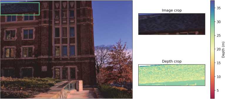
Fig. 1. Example of noisy region in the depth annotations in the DIODE dataset

The method presented in this work is designed to solve these problems. It enables the training of depth estimation models without relying on labeled real-world images, thereby avoiding the issues of noise and inaccuracies from measurement sensors.

1.    Related work

To circumvent the fundamental challenge of data collection, two main research directions have emerged: (i) selfsupervised learning from unlabelled videos or images [12], and (ii) the use of photorealistic synthetic datasets with perfect ground truth [13].

The first approach, self-supervised learning, aims to extract training signals directly from unlabeled real-world images. For example, Structure-from-Motion (SfM) [14] algorithm can analyze consecutive frames in a video stream to reconstruct a (typically sparse) scene structure and then it can be used to supervise a neural network. A similar idea can be applied to large image collections scraped from the Internet to generate training data. This allows for the automatic generation of depth maps, eliminating the need for expensive annotation.

A notable example is the MegaDepth dataset [15], which was generated by applying modern SfM techniques to a large collection of internet images. The primary advantage of this approach is its ability to use existing, readily available real-world images. However, it suffers from significant drawbacks: the resulting ground truth is often sparse, covering only static and well-textured areas of an image [14]. It can also be noisy and contain outliers in uniform or dynamic regions [15]. Most critically, the depth is estimated at an unknown metric scale, making it relative and requiring further calibration [16].

The second approach involves using synthetic datasets. These are typically created for a specific domain and consist of diverse, photorealistic images with pixel-perfect ground truth and known camera parameters. Synthetic data can model rare and complex scenarios, and the size of the dataset can be scaled as needed. The value and potential of this approach are underscored by the growing number of synthetic datasets [15 – 19] and their widespread adoption in monocular depth estimation research [20 – 23].

A primary limitation of this approach is the "sim-to-real gap"– the discrepancy between the data distributions of the real and simulated worlds that persists even with highly realistic rendering [26]. This gap can be minimized if a sufficient amount of unlabeled real-world data from the target domain is available. This is achieved through domain adaptation techniques, which transfer knowledge learned from a label-rich source domain (e.g., synthetic data) to a target domain where labeled data is scarce or nonexistent.

While there are many ways to classify these techniques, they can be conceptually divided into two main categories based on the level at which the domain distributions are aligned [27]: feature-level adaptation and prediction-level adaptation. Feature-level adaptation aims to train a neural network to extract internal representations from real and synthetic images that are statistically indistinguishable. The goal is to make the early layers of the model, which are responsible for recognizing basic patterns like edges and textures, perceive both data types similarly. Foundational works in this area proposed minimizing statistical discrepancies such as the Maximum Mean Discrepancy (MMD) [28] or aligning covariance matrices (e.g., Deep CORAL) [28]. This encourages the subsequent layers, which produce the final prediction, to become domain-invariant. While this approach can yield high-quality results, it is often more complex to implement and tune.

A more pragmatic and common alternative is prediction-level adaptation [29], often referred to as pseudo-labeling. Instead of intervening in the model's intermediate layer activations, this method operates on its final output. A "teacher" model, trained on synthetic data, generates predictions for a set of unlabeled real-world images [30]. These predictions, while imperfect, are then used as ground truth labels to train a second "student" model. Due to its conceptual simplicity, ease of implementation, and proven effectiveness [22, 28], pseudo-labeling is considered a powerful tool for bridging the domain gap [31].

Despite its popularity, pseudo-labeling has a fundamental limitation: the performance of the student model is typically capped by the performance of the teacher. If the teacher, trained on synthetic data, produces depth maps with artifacts or low level of detail, the student will inevitably inherit these flaws. Research shows that modern relative depth models, trained on vast amounts of real-world images, often produce maps with significantly higher detail and structural accuracy than even fine-tuned metric models [1, 20]. Metric models trained on sparse LiDAR data tend to generate smoothed and less-detailed maps, whereas relative depth models excel at reconstructing sharp boundaries and fine details [32]. Although these models do not predict absolute scale, they demonstrate an impressive ability to capture scene geometry and achieve strong zero-shot performance [33]. They possess a fundamentally better "understanding" of real-world geometry.

2.    Proposed method

The primary objective of this work is to propose a method for training high-quality metric monocular depth estimation models for a specialized application domain. As previously mentioned, a key constraint is the absence of labeled real-world data from the target domain.

To address this task, we have the following components at our disposal:

A set of unlabeled real-world images: Images from the target domain for which metric depth needs to be predicted.

"Metric Teacher" Model: A neural network trained on a photorealistic synthetic dataset from the target domain. It can generate metrically correct depth maps, but its predictions may be smoothed, lack fine details, and contain various artifacts.

"Relative Teacher" Model: A neural network pre-trained on vast and diverse real-world image datasets. It generates structurally accurate and highly detailed relative depth maps.

As discussed in the literature review, the vast majority of existing domain adaptation approaches for metric depth estimation rely solely on a metric model to generate pseudo-labels. However, modern relative depth models capture more precise and detailed geometric information, such as fine textures and sharper object boundaries. We hypothesize that a predicted relative depth map, up to a linear transformation, is a better representation of the true scene geometry than a predicted metric map.

We propose a pseudo-labeling method that uses the predicted metric map as a source of scale information to calibrate the highly detailed relative depth map:

^ pseudo    $ ' ^drelative + ^t , (1)

where d _pseudo is the final metric pseudo-label, d _relat i _ve is the relative depth map, s is the scale factor, and t is the shift factor.

The task of finding the scale and shift parameters (s, t) is framed as a linear regression problem. As a baseline, we consider the method of least squares (MSE), which provides an analytical solution but is sensitive to outliers. A more robust alternative is the RANdom Sample Consensus (RANSAC) algorithm [34]. It is widely used in image analysis tasks such as the automatic alignment of tomographic volumes [35], document image processing [34], and its modern implementations are being actively optimized to solve problems like 2D homography estimation [36]. RANSAC iteratively generates transformation hypotheses from random subsets of point pairs and selects the hypothesis that best explains the largest number of points (inliers) within a specified error threshold.

The robustness of the estimation depends not only on the chosen algorithm but also on the strategy for selecting the data points for calibration. We explore two pixel selection approaches: using all available points, or using a subset of "support" points formed by the extreme percentiles of the depth distribution. This second approach excludes the central, often smoother, part of the distribution. Specifically, we use the 10th and 90th percentiles of the metric depth map as thresholds:

^{Т _}{ ^ ^ ^fll^d metric ^(l) — ^p10^(dmetric ) V ^dmetric^(l) >  ^p90^(dmetric ) ^}, (2)

where, T is the resulting set of support points, l is a pixel from the set of all image pixels fl, d _metr i _c (i) is the depth value of that pixel from the metric teacher's prediction, and p ₁₀ (d _metri_c ) and P 9o (d _metric ) are the 10th and 90th percentile values of the entire metric depth map, respectively. This selection creates a mask of the nearest and farthest points, which are used for a more stable calibration.

Our support point selection strategy relies on the metric depth map to identify the nearest and farthest points in the scene, which provide robust geometric constraints for calibration. Because the metric teacher was fine-tuned on synthetic data from the target domain, its predictions provide a consistent, albeit smoothed, representation of the scene's absolute scale. While relative depth maps offer superior structural detail, they lack a meaningful scale; their extreme percentile values might highlight regions of high-frequency texture rather than the actual nearest and farthest scene points. Using the metrically-correct depth map ensures that our support points are genuinely representative of the scene's overall depth range, leading to a more stable and accurate scale and shift estimation.

We will evaluate the proposed methods in two ways: (i) by directly comparing the generated pseudo-labels against the ground truth, which is treated as a held-out set and is not used during training; and (ii) by comparing the performance of neural networks trained on the pseudo-labels generated by the different methods.

3.    Experiments and results 3.1.    Experimental Setup

The KITTI dataset [37] with the standard Eigen Split [38] was chosen as the real-world dataset for our experiments. This dataset, captured in an urban environment using LiDAR for ground truth generation, is a standard benchmark for evaluating monocular depth estimation methods. The training set contains 23,000 images, and the test set includes 652 labeled images.

Our study involves three neural network models. Their roles and specifications are described in Tab. 1.

Tab. 1. Models used in the experiments

Role	Abbr.	Architecture	Description and Training Data
Relative Teacher	Trel	DepthAnything V2 Large	Foundational model trained on large-scale real-world datasets to produce structurally accurate relative depth maps [22]
Metric Teacher	Tmet	DepthAnything V2 Large	Fine-tuned on the synthetic VKITTI2 dataset [37] to generate metrically correct predictions in the target domain [22]
Student Model	° met	DepthAnything V2 Small	Compact model trained on the generated pseudo-labels to produce the final solution [22]

The quality of the predictions was assessed using a standard set of metrics for depth estimation:

Accuracy Metrics (51, S2, 63): These measure the percentage of pixels for which the model's prediction is sufficiently close to the true value within a certain threshold. Higher is better (T)

Error Metrics (AbsRel, RMSE, RMSE log): These measure the average discrepancy between predicted and true depth values across the entire image, in either absolute or logarithmic units. Lower is better (f).

• 3.2.    Direct Pseudo-Label Evaluation

The pseudo-label generation process begins with running both teachers on a source image. The calibration parameters are then determined to align the relative teacher's predictions. These parameters are calculated based on a set of pixels that can either include all image pixels or a subset of "support" points defined by the 10th and 90th percentiles of the metric depth distribution.

To evaluate effectiveness, five different configurations were established:

Baseline: Pseudo-labels are generated directly from the metric teacher's predictions without any calibration.

MSE: A hybrid method where calibration parameters for the relative depth map are determined using the least squares (MSE) method on all points.

Masked MSE: Similar to the above, but the regression is performed only on the subset of "support" points (10th and 90th depth percentiles).

RANSAC: A hybrid method that uses the outlier-robust RANSAC algorithm to find calibration parameters using all points.

Masked RANSAC: A combination of the RANSAC method with the "support" point selection strategy.

We configured our RANSAC implementation to perform a maximum of 1000 iterations. In each step, the algorithm constructed a hypothesis from a random sample of 50 points and classified points as inliers if their residual error was below a threshold of 0.1.

The first stage of experiments involved a direct quality assessment of the pseudo-labels generated by these methods by comparing them against the ground truth from the train and test KITTI Eigen Split. The results are presented in Table 2.

Tab. 2. Direct comparison of pseudo-label quality on the KITTI

Method	S i T	8 2 T	«3T	AbsRel f	RMSE I	RMSE log f
T mpt (Baseline)	0.773	0.953	0.990	0.171	4.406	0.199
MSE	0.806	0.962	0.991	0.152	4.501	0.186
Masked MSE	0.836	0.969	0.993	0.134	4.047	0.168
RANSAC	0.809	0.965	0.992	0.153	4.308	0.183
Masked RANSAC	0.836	0.970	0.994	0.134	4.043	0.167

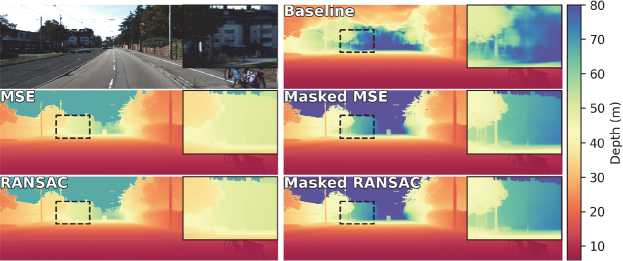
Fig. 2. Visual comparison of pseudo-label generation methods

The hybrid approaches, which use the structurally accurate relative depth maps from T _re[ , show a significant advantage over the baseline method. The Masked RANSAC method achieved the best results across all metrics, reducing the Absolute Relative error from 0.171 to 0.134 and the RMSE by from 4.406 to 4.043 compared to the Baseline. A visual comparison of the pseudo-labels generated by the different methods is presented in Fig. 2.

• 3.3.    Student Training on Pseudo-Labels

To provide a final validation of our method's effectiveness, a second experiment was conducted by training a compact student model (S _met ) on the pseudo-labels generated by different methods. The goal was to assess how improvements in pseudo-label quality translate to the final performance of the target model. We compared two sets of training data: pseudolabels from the baseline metric teacher (T_met) and those from the best-performing Masked RANSAC method.

^The S met model was trained for 120 epochs with a batch size of 32 and an initial learning rate of 5 • 10 ⁶. Data augmentation consisted of random horizontal flips with a probability of 0.5. The input image resolution was 196×644 pixels. The evaluation results on the KITTI Eigen Split test set are shown in Tab. 3.

Tab. 3. Performance of the S _met trained on different pseudo-labels

Training Labels	S j I	« 2 T	8 , 1	AbsRel f	RMSE f	RMSE log f
Tmet (Baseline)	0.815	0.959	0.989	0.151	4.032	0.181
Masked RANSAC	0.863	0.971	0.994	0.115	4.055	0.156

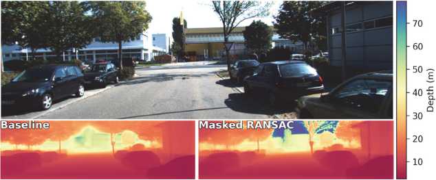
Fig. 3. Visual comparison of student models prediction

The results of this indirect comparison confirm the conclusions from the previous stage. The model trained on pseudolabels generated by the Masked RANSAC method demonstrates a significant superiority over the model trained on the baseline labels from T _met . The most substantial improvements are seen in the AbsRel (a 23.8 % reduction from 0.151 to 0.115) and RMSE log (a 13.8 % reduction from 0.181 to 0.156) metrics.

The fact that the baseline model shows a marginally superior RMSE merits some explanation. Firstly, the difference is negligible (approximately 1%), whereas our method demonstrates significant improvements across alternative metrics. Secondly, the relatively higher RMSE can be explained by the high sensitivity of RMSE to large outliers in distant regions. Our method produces sharper and more detailed depth maps, which can occasionally lead to significant errors on a small number of pixels at complex object boundaries. The lower RMSE log values obtained corroborates this observation, as the logarithmic metric is less sensitive to such sparse, large-magnitude errors.

A visual comparison of the results from the models trained on the baseline and the best-performing pseudo-labels is shown in Fig. 3. This experiment proves that enhancing the quality and detail of pseudo-labels by combining metric and relative model predictions directly translates into higher accuracy for the final model.

• 3.4.    Discussion

The experimental results validate our dual-teacher framework, confirming that hybrid pseudo-labels significantly improve model quality in the absence of annotated real-world data. The core of this success lies in robustly calibrating the structurally superior relative depth map using the metric teacher for scale information. Our analysis revealed that the most critical component of this process is our "support points" selection strategy. By focusing calibration on the nearest and farthest points in the depth distribution, this strategy leverages strong geometric constraints while avoiding noise from uninformative, uniform regions. The impact of this targeted selection proved more substantial than the choice between the RANSAC and MSE calibration methods. Despite this, RANSAC remains the theoretically preferred method due to its inherent robustness against outliers.

Conclusion

In this work, we proposed a method for training metric monocular depth estimation models that does not require labeled real-world data from the target domain. The approach aims to combine the fine-grained structure of relative depth with the absolute scale of metric depth by creating hybrid pseudo-labels.

We experimentally determine that the most effective calibration is achieved using the RANSAC algorithm applied to a subset of "support" points formed by the closes/farthest subsets of the depth distribution. A direct comparison on the KITTI dataset demonstrated that this method (Masked RANSAC) improves the quality of pseudo-labels compared to the baseline approach, reducing the AbsRel by 21.6 % (from 0.171 to 0.134) and the RMSE by 8.2 % (from 4.406 to 4.043).

Furthermore, a student model trained on the generated pseudo-labels significantly outperformed a model trained on the baseline labels, with improvements in AbsRel and RMSE log metrics of 23.8 % (from 0.151 to 0.115) and 13.8 % (from 0.181 to 0.156), respectively.

Our research proves that the proposed method is an effective solution to the domain adpatation of depth estimators. It enables the creation of domain-specific metric models with high level of detail for practical applications without the expensive process of collecting and annotating large volumes real-world data.