Reduced complexity FSD algorithm based on noise variance

Published Online December 2010 in MECS

Multiple-input multiple-output (MIMO) systems have been accepted as one of the most significant technology to improve the spectrum efficiency in wireless communications [1][2]. Nevertheless the detection of the MIMO is a big challenge for the application of MIMO systems. Maximum likelihood (ML) detection is able to provide the optimal performance, yet its calculation complexity is too big a burden for system especially with high modulation order and large antenna number [3]. The complexity of zero forcing (ZF) detection or minimum mean square error (MMSE) is low, but the performance is always bad. Several algorithms have been created to balance the conflict between the performance and the complexity. The V-BLAST algorithm has a little more calculation complexity than the ZF and MMSE algorithm, but its performance promotes a lot, especially combining with the ordering. The class of sphere decoding (SD) algorithm has been widely acknowledged as the one of the most promising algorithms [4][5]. K-best sphere decoding (K-best SD) algorithm is able to work in parallel and the computation complexity is constant, so that it attracts much attention [6]. However, to attain high performance with K-best SD, large K is needed, which causes the calculation complexity arising. The fixed sphere decoding (FSD) algorithm has been proposed to lower the complexity while maintain high performance and the parallel calculating ability of the K-best SD [7][8]. But, it is still necessary to further lower the complexity of the FSD without significant performance drop to meet the demand of the development of wireless communication. In this paper, a new algorithm to further reduce the complexity of the FSD is proposed.

The rest of the paper is organized as follows: Section II reviews the MIMO system. Section III reviews the related algorithm. The new algorithm is proposed in section IV. Its simulation results are shown in section V. At last, the conclusion is drawn in section VI.

II.    Mimo system

Consider a complex-valued baseband MIMO system with Nt transmit antennas and Nr receive antennas, where Nr ^ Nt, like Fig. 1. Assuming it is well in the complex domain.

Before further disposition, the channel matrix

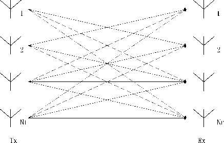
Fig. 1. MIMO system symbol-synchronous at the receiver, the received symbol can be written as

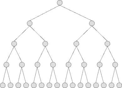
Fig. 2. Tree search and ML algorithm should be decomposed to triangular matrix.

y=Hx+n               (1)

^ ( H ) -3 ( H ) ³( H ) K ( H )

=QR

where x = [ x, x 2 ••• xNt ] T denotes the Nt -vector of the transmit symbol, y = [y, y2 ••• yNr ]T is the

Nr-vector    of the received symbol and where Q is a unitary matrix and R is an upper triangular matrix. Then (2) is left multiplied by QH to remove Q and to make the channel matrix triangular. Equation (3) will be expressed as n = [ n1 n 2 ••• nNr ]T   is the Nr -vector of the

ρ =Rs+η                 (5)

independent and identically distributed additive white complex Gaussian noise. H denotes the Nr X Nt Rayleigh fading channel matrix with h_i j ~ CN(0,1). For sake of simplicity, we set Nr = Nt = N /2. The ML detection is given by

where

n=Q H f- ( ⁿ ’

p=Q h " ' )

И y).

and

The ML algorithm can be expressed as

x ML = arg mⁱⁿ| |y — ^H x||² x eK

where К denotes the N/2-dimensional constellation lattice, like Fig. 2.

III.    FSD algorithm

A. Tree search and SIC algorithm

The variables in (2) are complex. The analysis is clear to be understood in real domain. So we transform (2) into

M y ) ) ta( H ) -3 ( H ) )Г^ ( X )WK ( n ) ) l<3 ( y № H ) * ( H )Д з ( x ) J (з ( n ) J ⁽⁾

s = arg min | |p -Rs| |2               (6)

n where Q is the real counterpart of К , s = (s, s2 ■■■ sN)T is the estimated value of transmit vector.

Equation (5) can also be written as

" P i Л P 2	—	r r , 0 M	r 12 r 22	r l N r 2 N		r V s 2 M	+	r n i ^ n 2 M	(7)
. P n >		ч 0	0	r NN >		ч SN >		ч n N >

From (7) , it can be found that

P n = r NN ^ ⁺ n N               ⁽⁸⁾

where ^ ( □ ) and 3 ( □ ) represent the real or the image

So sN can be calculated by part of (□). Certainly, the proposed algorithm can work

s N — round | P N- |                         (9) к r NN ) wh e re s ˆ N is the estimated transmit signal. Fig. 3. SIC algorithm Also from (7) , each transmit signal can be calculated recursively. , Г1 Г Г N _ VVV S; — round — p -     r t ^k           (10) к r l    к k ~1      ))) So the solution of (6) can be searched layer by layer. That is the principle of tree search and successive interference cancellation (SIC) algorithm are shown in Fig. 3. Each possible transmit signal s i is called a node in the searching tree. Each line from the top node is called a searching rout. The solid lines and nodes mean the solution of the SIC. B.    ML algorithm If the solution of a certain s i is wrong, the solutions of s j (when j) will almost always have errors. ML algorithm avoids it by calculating all the possible nodes in the tree, then selects the node which satisfies (6) from all the possible nodes. So the ML algorithm provides the best detection performance. C.    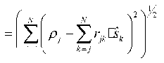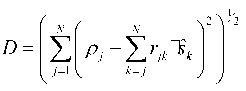Euclidean distance and the partial Euclidean distance The Euclidean distance (ED) between transmit and receive symbol is defined as Г N (      N      V )12 D = Z l Pj - Z j3k I            (11) к j =1 к       k = j         ) y Define the partial Euclidean distance (PED) as

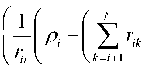
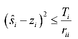
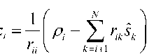
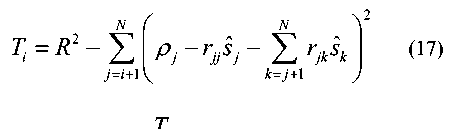
D — Z I P j - Z r* ^ J          (12) ( у = - Л      k - j        J) Obviously, the solution of (6) is to find the s ˆ with the smallest ED. D. The SD algorithm The main idea of the SD algorithm is to constrain the searching area to lower the complexity of the ML. A radius R around the receiver vector in the hyper-sphere is set first. So that the SD search can be represented as x s D = argmin y-Hx 2              (13) x eN y-Hx| |2 S R 2 After the triangular decomposition (4) , (13) can expressed as ||P - Rs|2 <  R                 (14) The solution to (14) can be got recursively using a depth-first tree search. Consider (7) , only a few nodes can be searched. They satisfy 2 T (- S/ - Zi ) < —                 (15) rii where 1 Г    N z / =- Р / - E r /ksk           (16) r i к       k - i + 1       ) and N Г                      V ' Ti = R - ^ P j - r jj s j - Z r jk s k     (17) j - i + 1 к                  k - j + 1        ) with zN — .? N and TN — R 2 . It is obvious that TN >  T n -1 > ... >  T 1                 (18) SD algorithm starts the search from the nodes on the top of the search tree to the leaf nodes (the nodes at the bottom of the tree). If a solution is found, the Euclidean distance of this route takes the place of the R as the new radius, and then new search continues on other routes until all routes are searched. If the R is set too small to find a solution in it, R should be adjusted larger to search again until a solution is found. But that is a bad situation because all calculation in the previous search is wasted. SD algorithm cannot run in parallel because the radius is

always renewed when any new solution is found.

The main idea of the K-best SD algorithm is to execute the search parallel. Also in the search tree, a certain number of routes are explored from the top to the

Therefore, the diagonal elements satisfy

E [ ^n ]< E [^ -1 ]<... <  E [ r 2 ]      (19)

Consider both (18) and (19) , we have

> E

T

² N -1

N -1, N -1

> ... >  E

T 1 r ²

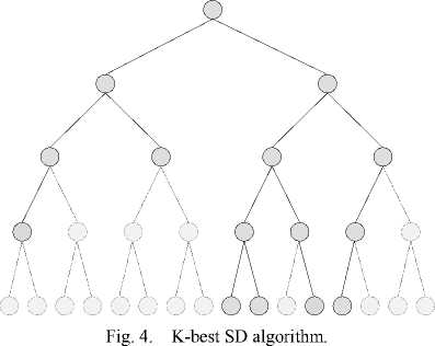
bottom at the same time. To lower the node number, only K nodes with the smallest PED are kept at each layer, like Fig. 4.

E. The K-best SD and FSD algorithm

The main idea of the K-best SD algorithm is to execute the search parallel. To lower the node number, only K nodes with the smallest PED are kept at each layer. To avoid performance dropping much, the number of K cannot be set small. That is why the complexity of the K-best SD is higher than that of the SD in the same performance. But the K-best SD attracts much attention because of the property of parallelism. Many works have been proposed to reduce the complexity of the K-best SD. One of the famous is the FSD algorithm.

Denote B i the candidate number of the child nodes at level i . For the K-best SD, B i =m ( m is the order of the modulation). Then the total number of the visited nodes is K X m for every layer. When the modulation order is high, the number of the visited nodes is a big number. That is a main reason why the complexity of the K-best SD is high.

The FSD explores the characteristic of the triangular matrix, and makes use of the fact that

• •    The diagonal elements of it have a Chi-square distribution with ( N-i+1 ) degrees of freedom.

• •    The off-diagonal elements are independent complex Gaussian random variables

r ij ~ CN (0,1).

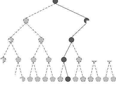
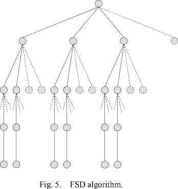
Consider both (15) and (20) , the average limited area becomes smaller and smaller. It is sure that the average number of nodes inside the limited area becomes smaller and smaller. So it is reasonable to reduce the candidate number of the node layer by layer. By this way, the FSD algorithm can drop the complexity of the K-best SD algorithm without large performance drop. For example, in a 4 X 4 system with 4-QAM modulation, the number of children nodes number per level can be B = ( B 1 B ₂ B 3 B ₄ ) T = ( 1 1 2 3 ) T , like Fig. 5.

Each element of the vector means the number of the visited children nodes of this layer. For example, B ₄ = 3 means the number of the visited children nodes for each node in layer four is three. The algorithm starts from the layer of the largest number, so the last number of B is always the largest one. The solid lines in figure mean the visited nodes. The dotted lines mean the children nodes which will be omitted. The corresponding calculation will be cut for these nodes and so the complexity will drop.

IV. Noise variance based reduced FSD algorithm

The complexity of the FSD is still high, so that works have done. Some works simplify the calculation by redesigning the ordering preprocessing [9][10]. [11] simplifies the calculation by reducing the numbers of kept routes. But the numbers are selected without strict proving. [12][13] simplify the calculation by setting a threshold which is calculated according to the intersection point of the probability distribution function (PDF) curves of xN2 and xN,Y2, where xN2 is the central chi-square distribution and xN Y2 is the non-central chi-square distribution. But that is the way to

balance the error of both χ_N ² and χ_{N , γ} ² when both two distributions are detected. So it is not the optimal threshold for only χ_N ² detection.

In this paper, we reduce the complexity of the FSD algorithm by explore the statistics property of the receive signal.

A.    Principle

The noise generates the bias between the receive signal and the product of the channel matrix and the transmit signal. The value of the noise variance determines mean square of the bias. So if the variance of noise is known, a threshold can be set to cut the node whose PED larger than it, like Fig. 6. Fortunately, when a channel condition is known, we can get the power of the noise. Given N receive antennas for a system, a pre-calculated radius, which is called pruning radius, can be set.

λ = βNσ ² (21)

where β is a tuning parameter to balance the performance and the complexity. Obviously, the larger the tuning parameter, the larger the pruning radius, the more number of nodes is kept and the less performance drop. On the contrary, the smaller the tuning parameter, the smaller the pruning radius and the more calculation reduced. So a real system can choose the appropriate value of tuning parameter according to the QoS requirement.

B.    The algorithm

The proposed algorithm is given as follows:

• 1)    Set β according to the toleration of performance drop and complexity, and then get pruning radius λ .

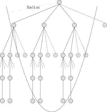
Fig. 6. Reduced FSD algorithm.

• 2)    The channel matrix is QR decomposed, and y is left multiplied by Q to get ρ .

• 3)    Set le=N

• 4)    Extend the surviving nodes to their children nodes according to the presetting expend number B i .

• 5)    le=le -1

• 6)    If le >1, go to step 4) .

• 7)    If le =1, select the node that has the smallest ED as the solution of the algorithm.

C.    Ordering

It is well known that the channel matrix ordering is a very useful preprocessing stage, which can significantly promote the performance. The V-BLAST algorithm orders the channel matrix so that the layer with the smallest noise power gain is detected first, the second detected layer with the second smallest noise power gain, and so on. This order guarantees the detection errors for the previous detected layers are smallest than that of the latter layers. The reason is because the algorithm detects layer by layer. If there happens any error in the previous layers, the later detection will be almost all wrong.

The famous V-BLAST ordering algorithm is

• •    for i=N,N-1,_,1

• •     G i = h;

• •      k i =argmini l^{( G} i ⁾ j

• •       H i = ( H i -1 ) k

• •    end

where H = ( H .). means that the k ,-th column of H

1 k should be set zero and Hit = (HHHi) HH .

There is a little difference between the above algorithm and the original V-BLAST ordering algorithm. In the latter, there are other steps for the cancellation of the interference. But the node number is not one for the former, it is impossible to cancel the interference for all nodes. Here we only keep the same part.

The previous detected layers have more impact on the performance than the later detected layers. So the number of the children nodes for the previous detected layers is often set as large as it can be. In many case, B = ( 1 1 1 4 ) T has better performance than

B = (1 1 2 2) T or B = (1 2 1 2) T . But in some cases, the children nodes’ number of the previous detected layer is set as large as possible so that it may be equal to the modulation order, or say the number of the constellation. There is no error propagation when all possible nodes are kept in a certain layer for further detection. So it is wasteful to set the noise gain small. On the contrary, the noise gain can be set as large as possible. The steps performed in the algorithm are the following.

• •    for i=N,N-1,...,1

• •    g , =h;

  I ( G i ) j | Г I ( G -j

  
  

  •

  
  

  k_i

  
  

argmax =< яk1...k-1} arg min

, je{ki-ki-1} if Bi = P if Bi < P

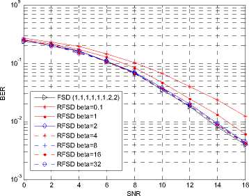
Fig. 7. Performance of RFSD in a 4×4 4QAM system.

• •    H i = ( H i -1 ) k

• •    end

where P is the maximum possible number of nodes, the number of the constellation. We choose this ordering algorithm in the proposed algorithm.

V.    Simulation Results

The proposed algorithm is compared with the FSD by the bit error rate (BER) and the computation complexity. Data are simulated in a 4 X 4 Rayleigh flat fading plus additive white Gaussian noise MIMO channel.

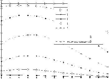
Fig. 7~12 show the performance and the complexity of the FSD and the noise variance based reduced FSD algorithm (RFSD in figures). Fig. 13~18 show those of the ordering FSD and the noise variance based reduced ordering FSD algorithm (ROFSD in figures).

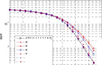
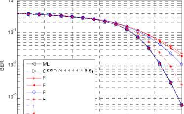
All the performance figures show the impacts on BER of different в . When в is large enough, the BER performance of the proposed algorithm is very close to that of the FSD. For example, When в = 32, 16, 8, the performance drop is hard to distinguish for the 64QAM modulation for both ordering and non-ordering FSD. In the figures showing the ordering algorithm, the difference between the proposed algorithm with в large enough and the ML algorithm is very small.

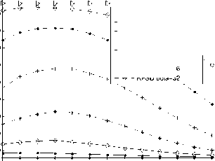
All the complexity figures illustrate the complexity of the proposed algorithm and the impacts on BER of different в • It can be found that, the number of reduced node is associated with the SNR and в • The percent of reduced node number arises according to the increase of SNR and drop of в • When the SNR is high enough, different lines tend to the same. When the SNR is high

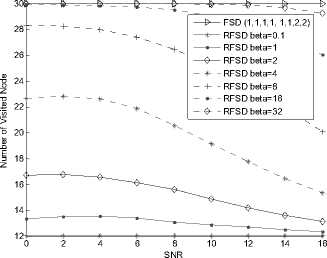
Fig. 8. Complexity of RFSD in a 4×4 4QAM system.

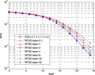
Fig. 9. Performance of RFSD in a 4×4 16QAM system.

0            5            10           15           20           25

SNR

FSD (1,1,1,1, 1,1,4,4)

RFSD beta=0.1

RFSD beta=1

RFSD beta=2

RFSD beta=4

RFSD beta=8

RFSD beta=16

RFSD beta=32

10-2

15       20

SNR

FSD (1,1,1,1,1,1,8,8)

RFSD beta=0.1

RFSD beta=1

RFSD beta=2

RFSD beta=4

RFSD beta=8

RFSD beta=16

RFSD beta=32

10-3

Fig. 10. Complexity of RFSD in a 4×4 16QAM system

Fig. 11. Performance of RFSD in a 4×4 64QAM system.

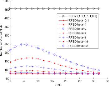
Fig. 12. Complexity of RFSD in a 4×4 64QAM system

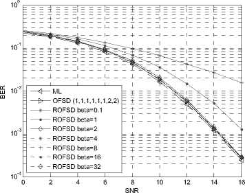
Fig. 13. Performance of order RFSD in a 4×4 4QAM system.

enough, different lines tend to the same. In Fig. 18, when SNR=30, the percent of the reduced nodes are about 82.9% when в = 0.1, 1 or 2. When в = 4,8, it becomes to about 82.4%, 81.2%. The percent turns to 77.6% or 69.1% when в = 16 or 32. From the complexity figures, it can be concluded that the reduced calculation becomes large when the modulation order arising.

VI.    CONCLUSION

This article proposed a new algorithm to reduce the calculation complexity of the FSD algorithm. According to the noise variance, a threshold can be set. A node who’s PED larger than it can be cut during the processing of tree search. To balance the performance and the complexity, a tuning parameter can be multiplied into the

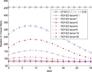
Fig. 18. Complexity of order RFSD in a 4×4 64QAM system

28 т"

OFSD (1,1,1,1, 1,1,2,2)

ROFSD beta=0.1

--•-- ROFSD beta=1

ROFSD beta=2

ROFSD beta=4

• -    + - ROFSD beta=8

• —    • — ROFSD beta=16

• -    0 - ROFSD beta=32

0       2       4       6        8       10      12      14       16

SNR

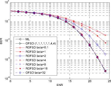
Fig. 15. Performance of order RFSD in a 4×4 16QAM system.

Fig. 14. Complexity of order RFSD in a 4×4 4QAM system

5            10            15           20           25

SNR

OFSD (1,1,1,1, 1,1,4,4)

ROFSD beta=0.1

ROFSD beta=1

ROFSD beta=2

ROFSD beta=4

--Н - ROFSD beta=8

• —    -• — ROFSD beta=16

• -    О - ROFSD beta=32

ML

OFSD (1,1,1,1,1,1,8,8)

ROFSD beta=0.1

SNR

ROFSD beta=1

ROFSD beta=2

ROFSD beta=4

ROFSD beta=8

ROFSD beta=16

- О - ROFSD beta=32

10-4 0

Fig. 16. Complexity of order RFSD in a 4×4 16QAM system

Fig. 17. Performance of order RFSD in a 4×4 64QAM system.

threshold. Simulation results in several scenes show that the algorithm can efficiently reduce the complexity of the FSD and maintain the performance.

Acknoledgement

This work is supported by NSFC Grant No.60972008.

Shubo Ren is the corresponding author.