Reducing Multicast Redundancy and Latency in Multi-Interface Multi-Channel Wireless Mesh Networks

Published Online October 2009 in MECS

Wireless Mesh Networks (WMNs) have been proposed to provide cheap, easily deployable and robust Internet access. A WMN is a multi-hop wireless network with a large number of mesh routers and mesh clients. The mesh routers in a WMN are usually static and can be equipped with multiple network interface cards (NICs). Furthermore, multiple non-overlapping channels can be available in the WMNs. For example, the IEEE 802.11b standard and IEEE 802.11a standard offer three and twelve non-overlapping channels respectively. Two mesh routers are able to communicate with each other as long as they are within the transmission range of each other, and one of their NICs uses the same channel [1] [2] .

Recently, there has been an upsurge of international interest in WMNs. Studies have been done on various

Manuscript received March 9, 2009; revised July 2, 2009; accepted August 15, 2009.

aspects of WMNs, such as topology control, QoS routing and channel assignment [1] . Nevertheless, the problems related to multicasting in WMNs have not been investigated much. The multicast/broadcast problems were studied mostly in single-channel wireless ad hoc networks. It was showed that the blind flooding approach can be very costly and can lead to serious redundancy, bandwidth contention and collision [13] . Therefore, quite a few multicast routing algorithms with better performance have been proposed in the literature, and most of them were based on trees or meshes [8] - [11] . However, all these algorithms took the assumption that there is only one channel available in the network, so they are not suitable for the multi-interface multi-channel WMNs.

Roy et.al. [4] showed that there was a fundamental difference between unicast and multicast routing in how data packets are transmitted at the link layer, and adapted certain routing metrics for unicast for high-throughput multicast routing. The main drawback of their work is that the utilization of multiple channels was not considered. Zeng et.al. [5] proposed a Level Channel Assignment (LCA) algorithm and a Multi-Channel Multicast (MCM) algorithm to optimize throughput for multi-channel and multi-interface mesh networks. Yuan et.al. [3] proposed a cross-layer optimization framework for throughput maximization in wireless mesh networks, in which the data routing problem and the wireless medium contention problem were jointly optimized for multi-hop multicast. However, both of the studies in [5] and [3] aimed at improving the multicast throughput in WMNs, and the problem of reducing the multicast redundancy was not investigated by them. Furthermore, none of the studies mentioned above investigated the multicast scheduling problem in WMNs.

In this research, we present an approach which jointly reduces the redundancy and latency for multicasting in multi-interface multi-channel WMNs. Han et.al. [6] pointed out that the problem of reducing the multicast redundancy in WMNs was very different from that in single-channel wireless ad hoc networks, for the redundancy of multiple NICs should be considered in a multi-channel environment. In this paper, we present two heuristic-based algorithms for low-redundancy multicast tree construction and low-latency multicast scheduling. Since broadcasting can be considered as a special case of multicasting, we also study the low-redundancy broadcast tree construction problem and propose an approximate algorithm with a constant approximation ratio. The main contributions of this paper are summarized in the following:

♦ The new concept of interface redundancy is presented, which concerns the number of NICs needed for multicasting/broadcasting in a multi-interface multichannel WMN. We prove that building a multicast/broadcast tree with the minimum interface redundancy is NP-hard, and propose a heuristic-based algorithm for multicast tree construction. We also present an approximate algorithm for broadcast tree construction with a constant approximation ratio.

♦ We prove that the minimum latency multicasting in a multi-interface multi-channel WMN is a NP-hard problem, and present a heuristic-based low-latency multicast scheduling algorithm. The scheduling algorithm is based on the low-redundancy multicast tree we build, so the multicast redundancy and latency are jointly reduced in our approach.

♦ Extensive experiments are conducted to test the algorithms we proposed, and the effectiveness of our approach is proved by the experiment results.

The rest of the paper is organized as follows. The network model and problem formulation is described in Section II. In Section III, we present the concept of interface redundancy and propose a heuristics-based algorithm for building a low-redundancy multicast tree. In Section IV, a low-latency multicast scheduling algorithm is proposed. In Section V, we study the problem of reducing the broadcast redundancy in a WMN. The simulation results of our algorithms are presented in Section VI. We conclude the paper in Section VII.

• II.    System Model and Problem Definition

We use a network model similar to that described by [2] [15] . We will use the notations introduced by [2] to represent the channel assignment and network topology. A multi-interface multi-channel wireless mesh network is modeled by an undirected connected graph G =( V,E ), where V represents the set of nodes in the network, E the set of edges(or links) that can carry data. There exist δ available non-overlapping channels in the network, denoted by the set {1, 2, ..., δ }. Each node v in V is equipped with Q ( Q _≤ δ ) radio interfaces (NICs).

We assume that all nodes in the network use the same fixed transmission power, i.e, there is a fixed transmission range ( r > 0) associated with every node. A channel assignment H assigns each node v ∈ V a set of Q different channels: H ( v )={ H 1 ( v ), H 2 ( v ),…. H Q ( v )}⊆ {1, 2, … . , δ }. The Q NICs at node v are tuned to the Q different channels in H ( v ) respectively. We assume a unit disk graph (UDG) model [16] . Each node has a known geographical location, and there exists an edge e =( u , v ; c )

on channel c between nodes u and v in V if and only if d ( u,v ) _≤ r and c ∈ H ( u ) ∩ H ( v ), where d ( u,v ) is the Euclidean distance between u and v . Note that G is a multi-graph, i.e., more than one edge may exist between a pair of nodes, because a pair of nodes may share two or more channels. If we merge the multiple edges between each pair of neighboring nodes of V into one edge, G will become a single graph, which is denoted by S ( G ). We assume that there are no vacant NICs, i.e., any NIC of each node is tuned to a channel that is shared by the NIC of a neighboring node.

We assume that time is discrete, and there are totally y messages to transfer from a source node to a group of destination nodes. Since all the NICs have the same transmission rate, we assume without loss of generality that each message can be transmitted in one time slot on any channel. When a node u transmits a message by one of its NIC tuned to certain channel c , any of u ’s neighbors equipped with a NIC tuned to the channel c can receive the message. If a node u hears multiple messages on the same channel c , we say that there is a collision at node u on channel c. A node u receives a message collision-free if u hears the message on certain channel without any collisions. In this study, we assume that the channel assignment work is done independently from our multicasting framework. The problem of channel assignment for multicasting performance improvement is interesting; however, it is out of the scope of this paper and will be the topic of another research work.

Let a WMN G= be given. Let r 0 be a source node in V . Let DN= { r 1 ,r 2 …r n } be a set of destination nodes in V 。 Our multicast problem is to find a routing and scheduling scheme to transfer y messages {1,2… y } from r₀ to the destination nodes in DN . The messages should be received in their original order (i.e, from 1 to y ) by every destination node. There are two sub-problems which we will study in such a process: (1) How should we define the multicast/broadcast redundancy of transmissions in such an environment? Can we minimize the multicast redundancy? (2) How to design a collision free scheduling scheme when the multicast redundancy is reduced? Can the multicast latency be minimized? In the following sections, we will present our solutions for these problems.

• III.    Reduce the Multicast Redundancy in a Wireless Mesh Network

In a single-channel wireless ad hoc network where every node has an omni-directional antenna, all the neighbors of a node can receive the same message by a single transmission. So minimizing the redundancy of multicast transmissions leads to building a multicast tree with the minimum number of forward nodes. This problem was proved to be NP-hard and some approximate algorithms were proposed [14] .

In a multi-channel WMN, however, a node u can transmit data to its neighbors though multiple channels. In such a case, not only should the redundancy of the forward nodes be considered, but also the redundancy of the forward NICs should be considered. This can be explained by a simple example in Fig.1. In Fig. 1, each node is equipped with three NICs, and the numbers written on each link denote the common channels between the link’s two endpoints. Suppose that the node A needs to send messages to D, E, and F, and there are two different multicast trees T1 and T2. We can see that in T1 at least three NICs are needed for node B to transmit a message to its neighbors D, E and F, whereas in T2 only one NIC is needed for node C to transmit a message to D, E and F. Since the NICs are usually costly resources, reducing the number of NICs needed for multicasting should be considered. Therefore, we introduce the concept of the “interface redundancy” of a mesh router:

Definition 1 ( The Interface Redundancy of a Mesh Router (IRMR)) Given a node u ∈ V and a set of u’s neighboring nodes N. Let K= { c | ∃ v ∈ N, and c ∈ H ( u ) I H ( v )} ( i.e. K is the set of all the common channels between node u and the nodes in N ) . Let a collection of N’s subsets be { { v | v ∈ N and c ∈ H ( v )} | c ∈ K } , The interface redundancy of u with respect to N is defined as the cardinality of the minimum set cover for N, and is denoted by cus ( u,N ) .

Given a multi-interface multi-channel wireless mesh network G which is defined in Section II . A multicast tree T m is a sub-tree of S ( G ) in which the source node r 0 is the root of T m , and each node in DN is a node of T m . We denote the sons of a node u in T m by sons ( u ), and denote all the non-leaf nodes of T_m by Rl ( T_m ). In Definition 2 we will introduce the interface redundancy of a multicast tree T m , which is defined as the sum of the interface redundancies of the non-leaf nodes in T m :

Definition 2 ( The Interface Redundancy of a Multicast

Tree(IRMT)) Given a multicast tree Tm of G. The interface redundancy of Tm is denoted by Cus(Tm), and

∑

Cus ( T m ) =

cus ( u,sons ( u ))

u ∈ Rl ( T_m )

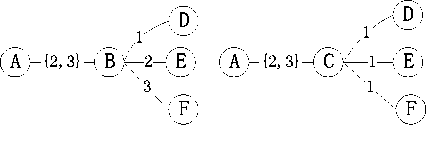
Figure 1. Muticast tree T1 (the left one) and T2 (the right one).

For example, see the two multicast trees T1 and T2 in Fig.1. The interface redundancy of the node B in T1 (with respect to the neighboring nodes { D,E,F }) is three; and the interface redundancy of T1 and T2 are four and two, respectively. Therefore, the multicast redundancy of T1 is greater than T2 , although T1 and T2 has the same number of forward nodes.

Our aim is to build a multicast tree with the minimum interface redundancy. However, this problem is NP-hard, as proved in Theorem 1:

Theorem 1 . Given a multi-interface WMN G. Building a multicast tree of G with the minimum interface redundancy is NP-hard.

Proof : Consider a special case where the set of destination nodes DN=V – { r 0 } , and all the nodes in DN are neighboring nodes of r 0 . In this case, we have

∑ cus ( u,sons ( u ))=cus( r₀ , DN ). At this time, building u ∈ Rl ( T m )

a multicast tree with the minimum redundancy equals to finding a Minimum Set Cover(MSC) for DN . The MSC problem has already been proved to be NP-hard [14] . Therefore, our problem is also NP-hard. □

Since building a multicast tree with the minimum interface redundancy is a NP-hard problem, we present a heuristic-based algorithm for it, as shown in Algorithm 1. The set of neighboring nodes of u is denoted by Ng ( u ). Algorithm 1 adopts a greedy strategy to select the multicast tree nodes in a bottom up way. The set of nodes which are i distance away from the source node is denoted by LL ( i ) , and the algorithm selects some nodes in LL ( i-1 ) as tree nodes after the nodes in LL ( i ) are selected. The criterion for node selection is: the node with the maximum ratio of neighboring tree nodes to interface redundancy is selected firstly (step 7). This criterion involves calculating the interface redundancy of a node, which is actually computing a minimum set cover (see Definition 1). Since the set cover problem is NP-hard [14] , we use a simple greedy approximate algorithm to calculate the interface redundancy of a node (see the Procedure CUS ( u,N )) .

Algorithm 1: Constructing a multicast tree with low interface redundancy

Input: A WMN G=, a source node r₀ and a set of destination nodes { r ₁ ,r ₂ …r _n}

Output: A multicast tree T_m with low interface redundancy

• 1.    Traverse G from r₀ using BFS until all the destination nodes are visited ( suppose the max level is k ) , and let LL ( i ) denote the set of nodes visited at level i.

• 2.    Add all the nodes in LL ( k ) to T_m;

• 3.    SEL^V Г о, Г 1 ,Г 2 ,Г з -.Г п } ;

• 4.    From i=k-1 to 0 Do {

• 5.    C ^ LL(i+1) I SEL;

• 6.    While C ≠ ∅ Do {

• 7.    u^ Arg max _{u G LL} ( i ) ( |Ng ( u ) I C/CUS ( u,Ng ( u ) I C )) ;

• 8.    Add the node u to T_m;

• 9.    Construct a link from u to every node in Ng ( u ) I C;

• 10.    SEL^ SEL U V u } ;

• 11.    C ^ C - ( neighbor ( u ) I C ); }}

• 12.    Return T_m;

• 13.    Procedure CUS ( u, N )

• 14.    Input: node u and a set of u’s neighboring nodes N;

• 15.    Output: approximate value of the interface redundancy

• of u with respect to N;

• 16.    s =0;

• 17.    While N≠ {} Do {

• 18.    c^ Argmax c e H _u ) ( | { v|v G Nandc G H ( v )} | );

• 19.    s++;

• 20.    N^N- { v|v G Nand c G H ( v )} ; }

• 21.    Return s;

• IV.    Low Latency Multicast Scheduling

The multicast latency is defined as the time interval from the first transmission to the first time at which every destination node gets all the messages. To reduce the multicast latency, an intelligent scheduling algorithm is needed. However, the minimum latency multicast scheduling in a WMN is a NP-hard problem, as proved in Theorem 2:

Theorem 2. The minimum latency multicast scheduling in a multi-interface multi-channel WMN is a NP-hard problem.

Proof. Consider a special case where the set of destination nodes DN=V – { r 0 } , and each node is equipped with only one NIC, and there is only one channel available in the network. In this case, our problem becomes the MLBS problem in [12] and [7] , which was proved to be NP-hard. So Theorem 2 holds'. □

We propose a heuristic-based algorithm for the low-latency multicast scheduling, as shown in Algorithm 2. Our scheduling algorithm is based on the multicast tree built by Algorithm 1. This is because that the NICs are used more effectively in a multicast tree with smaller interface redundancy, so the multicast latency tends to be reduced. For example, suppose the node A in Fig.1 has three messages to send to the destination nodes D , E , and F . A simple calculation reveals that the smallest multicast latency of T1 and T2 are five and four, respectively. Therefore, the multicast tree ( T2 ) which has the smaller interface redundancy also has the smaller multicast latency.

The output of Algorithm 2( TSch ) is a set of 4-tuples, and each tuple ( sn, sm, sc,t ) denotes that node sn will transmit message sm on channel sc at time slot t . We assume that each node has a message queue which caches the messages to be sent. In Algorithm 2, Msg ( u,t ) denotes the set of messages which are received before time t and are stored in the message queue of node u ; FC ( u,t ) denotes the set of collision-free channels that can be used by node u at time slot t ; NTS ( u,i ) denotes the set of neighboring nodes of u which have not received the message i ; Sons ( u,c ) denotes all the sons of node u in the multicast tree that have a common channel c with u .

At each time slot t, Algorithm 2 calls the procedure GetSelection repeatedly. The procedure GetSelection returns a tuple ( sn, sm,sc,rv ), which denotes that the selected node sn should transmit message sm on channel sc , and the nodes in the set rv will receive the message sm . After the tuple ( sn, sm,sc,rv ) is got, the SetInterfere procedure is called to change the collision-free channels of each node, because any other transmissions on channel sc at time slot t should not cause an collision to sn.

In the procedure GetSelection, a greedy strategy is adopted. That is, the criterion for selecting the tuple (sn, sm,sc,rv) is that the number of nodes in rv is maximal(step 17-21). The message sm is selected as the schedulable message which has the minimum message id(step 14-15). This guarantees that the destination nodes can receive the messages in their original order.

When the node sn transmit a message on channel sc , any node which has a common neighboring node with sn will not be able to transfer any data on channel sc at time slot t , because this will cause a collision. Besides, the nodes in rv are not able to transfer any data on channel sc at this time. Therefore, the channel sc is removed from the collision-free channels of these nodes, as shown in the procedure SetIntefere.

Algorithm 2: Low-latency multicast scheduling algorithm

Input：   the WMN G; the multicast tree Tm(the root is r0); y messages to send: {1,2….y};

Output ： the transmission schedule TSch;

• 1.    put the y messages into the message queue of node r₀;

• 2.    t^0; /*initialize*/

• 3.    While ∃ u ∈ T_m has not received all the messages Do {

• 4.    For each non leaf node u G T m Do { FC(u,t)^ H (u); }

• 5.    While ∃ u ( FC ( u,t ) ≠ ∅ ∧ Msg ( u,t ) ≠ ∅ ) Do {

• 6.    ( sn, sm, sc, rv ) ^ GetSelection ( G, T_m,t ) ;

• 7.    If ( |rv|=0 ) Then break;

• 8.    Else { add sm into the msg. queues of the nodes in rv; }

• 9.    SetInterfere ( sn,sm,sc,rv, t ) ;

• 10.    Add ( sn,sm,sc,t ) to TSch; }

• 11.    t++; }

• 12.    Return ( TSch ) ;

• 13.    Procedure GetSelection ( G, Tm,t )

• 14.    Let TS be the set of nodes which have messages in their messge queues and have collision- free channels to use at time slot t;

• 15.    sm ^Min { m G Msg ( u,t ) | u G TS } ;

• 16.    Candidates ^ { u G TS | sm G Msg ( u,t ) } ;

• 17.    For every u ∈ Candidates Do {

• 18.    cl ( u)^ Arg max _{c G FC} ( u ) ( | Sons ( u,c ) I NTS ( u,sm ) | ) ;

• 19.    nt ( u ) ^Sons ( u,cl ( u )) I NTS ( u,sm ) ; }

• 20.    sn F Arg maX u G Candidates ( |nt ( u ) | ) ;

• 21.    sc ^ cl ( sn ) ; rv^ nt ( sn ) ;

• 22.    If all the neighbors of sn in T_m have received the message sm Then {

• 23.    remove sm from the message queue of sn; }

• 24.    Return ( sn, sm, sc, rv ) ;

• 25.    Procedure SetInterfere ( G,Tm, sn,sm,sc,rv, t )

• 26.    Let N be the set of nodes in T_m which have a NIC tuned to channel sc;

• 27.    Let S be the neighboring nodes of sn in G;

• 28.    P ^{’w| Э u G S and w is a neighbor of u in G} I N;

• 29.    Q^ { sn } U rv U P

• 30.    For each node u G Q Do { FC(u,t) ^ FC ( u,t ) - { sc } ; }

• V.    Reduce the Broadcast Redundancy

The concept of interface redundancy of a multicast tree can be extended to the broadcasting case, since broadcasting is a special case of multicasting. However, there are subtle differences between a multicast tree and a broadcast tree. In a broadcast tree, a “broadcast backbone” can be constructed by the nodes whose degree is greater than one, and the number of different channels used by the “backbone nodes” should be reduced. Therefore, the concept of IRMT should not be applied directly in the broadcasting scenario, and we introduce the new concept of interface redundancy of a broadcast tree in Definition 3:

Definition 3: (The Interface Redundancy of a Broadcast Tree(IRBT)) Given a wireless mesh network G=(V,E), a broadcast tree Tb is a sub-tree of G that contains all the nodes in V. The interface redundancy of Tb, denoted by R(Tb), is the sum of the number of channels selected by the nodes in Tb whose degree is greater than one, i.e., R (Tb) =      ∑      |{k|∃(u,v;k)∈Tb }| u∈ Tb ∧ degree(u)>1

Not surprisingly, finding a broadcast tree with the minimum interface redundancy is also a NP-hard problem, as shown in Theorem 3:

Theorem 3 : Let T* be a broadcast tree of G such that R ( T* ) is minimal. T* is called a MIRB tree of G . Finding T* is a NP-hard problem.

Proof: Consider a special case in which every node is equipped with just one NIC. In such a case, we can see that the interface redundancy of any broadcast tree equals to the number of non-leaf nodes in the broadcast tree. At this time, finding a MIRB tree equals to the problem of finding a Minimum Connected Dominating Set (MCDS) of G . The MCDS problem has been proved to be NP-hard [14] . So finding a MIRB tree is also NP-hard. □

In the following, we will propose an approximate algorithm for finding a MIRB tree. Our approximation algorithm can be decomposed into two logical steps:

• 1)    Graph Transformation : In this step, we transform the original wireless mesh network graph into a new graph called “Shadow Graph” according to some transformation rules. We then prove that finding a MIRB tree in the original graph equals to finding a “Minimum Core Set” in the Shadow Graph.

• 2)    Computing a Minimum Core Set : In this step, we compute a Minimum Core Set in the Shadow Graph approximately. An approximate MIRB tree can be constructed based on the Core Set we computed.

• A.    Graph Transformation

In this step, we transform the wireless mesh network into a Shadow Graph, which is not a multi-graph. The rules for constructing a Shadow Graph are given in Definition 4:

Definition 4 : (Shadow Graph) The Shadow Graph of G, denoted by W ( G ) , is constructed by the rules described below:

• i)    For each node u in V, create a node in W ( G ) , which is denoted by w ( u ) . The node w ( u ) is called the shadow node of u. For each channel H j ( u ) in H ( u ) ( 1 ≤ j ≤ Q ) , create a node in W ( G ) , which is denoted by w ( u, H j ( u )) . The node w ( u, H j ( u )) is

labeled with the value of H j ( u ) , and is called the channel node of u on channel H j ( u ) . The set { w ( u,H 1 ( u )) ,w ( u,H 2 ( u )) ,...,w ( u,H Q ( u ))} is denoted by W l ( u ) .

• ii)    For each node u in V, construct an edge between each pair of nodes in W l ( u ) ∪ { w ( u )} . That is, the sub-graph induced by the nodes in W l ( u ) ∪ { w ( u )} is a clique. For any node i in W _l ( u ) ∪ { w ( u )} , u is called the primal node of i.

• iii)    For each edge ( u,v;c ) in E, construct three undirected edges in W ( G ) , which are ( w ( u,c ) , w ( v,c )) , ( w ( u,c ) , w ( v )) , and ( w ( u ) ,w ( v,c )) . For each edge e in {( w ( u,c ) ,w ( v,c )) , ( w ( u,c ) , w ( v )) , ( w ( u ) ,w ( v,c ))} , the edge ( u,v;c ) is called the primal edge of e. ( We assume that the primal edge of each edge constructed in ii) is null. )

We assume that each node in W ( G ) has a geographical location, which is the same as the location of its primal node. Note that W ( G ) is not a unit disk graph. This is because that for any adjacent nodes u,v V , w ( u ) and w ( v ) are not adjacent in W ( G ).

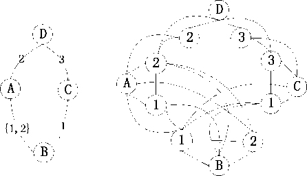
Fig.2(b) shows the Shadow Graph transformed from the wireless mesh network given in Fig.2(a). The four nodes A,B,C and D in Fig.2(b) are the shadow nodes of the four nodes in Fig.2(a), respectively. The other nodes in Fig.2(b) are the channel nodes.

(a)                              (b)

Figure 2. A wireless mesh network and its Shadow Graph.

According to the constructing rules of the Shadow Graph, the channels selected in a broadcast tree can be mapped to a set of channel nodes in W ( G ), which has some special properties. We clarify this by introducing the concept of Core Set:

Definition 5. (Core Set) Let S be the set of all the shadow nodes in W ( G ) . A Core Set K of W ( G ) is a set of channel nodes in W ( G ) that satisfies the following conditions:

• i)    The sub-graph induced by K is connected.

• ii)    For each node s S, there exists a node in K which is adjacent to s.

A Minimum Core Set is a Core Set of W ( G ) with minimum cardinality .

Theorem 4 proves that the size of a Minimum Core Set equals to the interface redundancy of a MIRB tree:

Theorem 4 . Let opt be a Minimum Core Set of W ( G ) . Then R ( T* ) = |opt|.

Proof. Our poof is formed by two parts: Part 1 proves | opt | ≤ R ( T* ), and Part 2 proves R ( T* ) ≤ | opt |:

• i)    Part 1:

Consider the set P ={ w ( u,k ) | ( u,v ; k ) ∈ T* and u is a non-leaf node in T* }. Apparently |P|= R ( T* ). We have:

• (a)    For any two nodes w ( u , k₁ ) and w ( u , k₂ ) in P ( k1 ≠ k2 ), we can know that they are connected in W ( G ), because the sub-graph induced by W _l ( u ) is a clique(according to the second rule in Definition 4).

• (b)    For any two neighboring non-leaf nodes u 1 and u 2 in T* and the edge ( u₁,u₂ ; k₃ ) in T* , there must exist an edge between w ( u 1 , k 3 ) and w ( u 2 , k 3 ) in W ( G ) (according to the third rule in Definition 4).

• (c)    For any node u in V , there must exist a node v and an edge ( u,v ; k ) in T* . If u is a non-leaf node in T* , then the shadow node w ( u ) must be adjacent to the node w ( u , k ) which is in P (according to the second rule in Definition 4). If u is a leaf node in T* , then v must be a non-leaf node in T* , and the shadow node w ( u ) must be adjacent to the node w ( v , k ) which is in P (according to the third rule of Definition 4). Therefore, there always exist a node in P which is adjacent to w ( u ).

From ( a ) and ( b ) described above, we can know that the sub-graph induced by P is connected. Thus the first condition in Definition 5 is satisfied by P . From ( c ), the second condition of Definition 5 is satisfied by P . Therefore, P is a Core Set of W ( G ). Since opt is a Minimum Core Set of W ( G ), we have: | opt | ≤ | P |= R ( T* ).

• ii)    Part 2:

Find all the primal nodes of the nodes in opt , and let the set of these primal nodes be denoted by M . Find any spanning tree Z of the sub-graph induced by opt ∪ { w ( u ) | u ∈ V - M }. Let G’ be the sub-graph induced by the primal edges of Z ’s edges. Through a similar reasoning with Part 1, we can know that G’ is a connected graph, and there exists a broadcast tree T ’ which is an arbitrary spanning tree of G’ . Besides, each channel selected by a non-leaf node in T’ corresponds to a channel node in opt . Therefore, we have R ( T’ ) ≤ | opt |. Since T* is a broadcast tree with the minimum interface redundancy, we have: R T* ) ^ R T’ ) ^1.        _П

Note that Part 2 in the proof of Theorem 4 actually provides a method to construct a broadcast tree from a Core Set.

• B.    Computing a Minimum Core Set

Note that the concept of Minimum Core Set is different from MCDS. The nodes in W(G) are partitioned into two disjoint sets: the set of shadow nodes and the set of channel nodes. The nodes in a Minimum Core Set are all channel nodes, and they must dominate all the shadow nodes. However, in the MCDS problem, all nodes are treated uniformly [14]. To make matters worse, the Shadow Graph is not a unit disk graph, as we mentioned before. Therefore, the previous algorithms for computing MCDS (both in general graphs and in unit disk graphs) cannot be applied in our case.

We give an approximation algorithm for computing a Minimum Core Set in Algorithm 3:

Algorithm 3: Computing a Minimum Core Set

( Step 1 ) Let Y be the sub-graph induced by all the channel nodes in W ( G ). Find a maximal independent set D in Y .

( Step 2 ) Assign each edge in Y a weight of 1. Find a Steiner Tree X in Y for connecting the nodes in D ( A Steiner Tree is a minimum weight tree connecting a given set of vertices in a weighted graph ). Let the set of nodes in X be denoted by X v . Then X v is the output of Algorithm 3.

The correctness of Algorithm 3 is proved by Lemma 1:

Lemma 1. X v is a Core Set of W ( G ) .

Proof. Apparently, the sub-graph induced by X_v is connected. For any node u in V , there must exist a channel node c in W l ( u ) such that c is adjacent to w ( u ). If c is not in X v , there must exist a node c’ in D which is adjacent to c (because D is a MIS in Y ). Since D is a subset of X v , c’ is also in X v . According to the rules in Definition 4, c ’ must be adjacent to w ( u ). Therefore, there always exists a node in X v ( c or c’ ) which is adjacent to w ( u ). According to Definition 5, X v is a Core Set of W ( G ). □

To analyze the performance bound of Algorithm 3, we will introduce the concept of Dominating Area, which corresponds to the channels assigned to a node and its neighboring nodes:

Definition 6 . (Dominating Area) Let c be any channel node in W ( G ) . Let u be the primal node of c. The Dominating Area of c, denoted by N ( c ) , is the set of channel nodes which correspond to the channels assigned to u and the neighboring nodes of u. i.e.: N ( c )=       U       W l ( v )

v = u or v is adjacent to u

Based on the concept of Dominating Area, Lemma 2 to Lemma 4 finds the relationship between the size of D and the size of opt :

Lemma 2. Let c be any channel node in W ( G ).There are at most 5 δ independent nodes in N ( c ).

Proof. The set N ( c ) can be partitioned into 5 mutually disjoint subsets, denoted by N 1 ( c ), N 2 ( c ), N 3 ( c ), ... ,

N ( c ). Each node in N j ( c ) has a label j (K j ^ 5 ). From our network model and the construction rules of W ( G ), it can be known that the sub-graph induced by N j ( c ) is a unit disk graph(1 ≤ j ≤ δ ). The nodes in N j ( c )(1 ≤ j ≤ δ ) are in the unit disk centered at c , so there are at most five independent nodes in N j ( c ) [17] . Therefore, there are at most 5 5 independent nodes in N ( c ). □

Lemma 3. For any channel node c in W ( G ), there must exist a node i in opt such that c is in N ( i ).

Proof. Let v be the primal node of c . Since opt is a Core Set, there must exist a node i in opt such that i is adjacent to w ( v ). If i is in W l ( v ), then c is in N ( i ). If i is not in W l ( v ), the primal node of i must be adjacent to v according to the construction rules of W ( G ) in Definition 4. Therefore, c is in N ( i ) according to Definition 6. □

Lemma 4. |D| ≤ 5δ|opt|.

Proof. From Lemma 3, we know that D can be partitioned into a number of mutually disjoint subsets the nodes in each subset are in the Dominating Area of certain node in opt. Since the nodes in D are mutually independent, from Lemma 2 we know:

| D | ^£ j e _opt 5 5 =5 5 | opt |      □

Lemma 5 and Theorem 5 find the approximation ratio of Algorithm 3:

Lemma 5. There exists a tree Z in Y which contains all the nodes in D, and there are at most 2 | D|+|opt| nodes in Z.

Proof. Let set P be initialized to D opt. For any node d in D and the primal node u of d , there must exist a node c in opt such that c is adjacent to w ( u ). From the rules in Definition 4, it can be known that there must exist a channel node d’ in W l ( u ) such that c is adjacent to d’ . Note that both d’ and d are in W l ( u ), so either d’ equals to d or d’ is adjacent to d . We add the node d’ into P . Therefore, when all the nodes in D are checked, there are at most 2 | D|+|opt| nodes in P , and the sub-graph induced by P is connected. Let Z be any spanning tree of the subgraph induced by P. So Lemma 5 holds. □

Theorem 5. |X_v| ≤ ( 20δ+2 ) |opt|-1.

Proof . From Lemma 5, we can know that a Steiner Tree in Y for connecting the nodes in D has at most 2| D |+| opt |-1 edges. In Algorithm 3, an approximation Steiner Tree algorithm such as that proposed in [18] or [19] can be used for computing X . The approximation ratio of the algorithm proposed in [18] or [19] is 2. So we have:

| X v | ≤ 2(2| D |+| opt |-1)+1

2(10 5 1 opt |+| opt |-1)+1=(20 5 +2)| opt |-1      □

We can construct a broadcast tree T from Xv using the method provided in the proof of Theorem 4. The interface redundancy of T will be less than |Xv|. Since in Theorem 4 we have proved that |opt|= R(T*), the interface redundancy of T will be at most (20δ+2)R(T*)-1. Finally, Algorithm 3 can also be implemented in a distributed way, and the interested readers are encouraged to refer to [20].

VI.    Experimental Evaluation

In this section we evaluate the performance of our algorithms via simulations. The experiments focus on the effect of various network conditions on the multicast tree’s interface redundancy(IRMT) and the multicast latency. In each experiment, we generate 120 network nodes randomly in a square, and the square’s length is set to 2km. We choose a node as the source node, and randomly choose some other nodes as the destination nodes. We choose the transmission range to be 300 meters, and the total channel number to be 10. The number of messages to transfer is set to 10. The channels are assigned to each node’s NICs randomly.

20 40 60 80 100 120

Number of Nodes

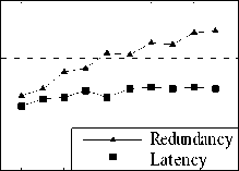
Figure 3. Interface redundancy and multicast latency vs. number of nodes

In Fig.3, we study the impact of the number of nodes on the multicast tree’s interface redundancy and the multicast latency. The number of each node’s NICs is set to 3, and we varied the number of destination nodes from 20 to 110 in steps of 10. The destination nodes are selected randomly. The multicast tree will have more nodes when the number of destination nodes increases, so the interface redundancy shows an uptrend. However, the interface redundancy does not strictly increase when the number of nodes increases. This is because the interface redundancy is influenced not only by the nodes of the multicast tree, but also by the channel assignment of each node (The channel assignment is done in a random manner in our experiments). From Fig.3 we can also see that the latency does not vary much when the destination nodes increase. This is because the maximal BFS levels of the destination nodes do not vary much in the settings of Fig.3.

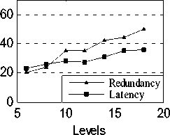
Figure 4. Interface redundancy and multicast latency vs. BFS levels

Fig.4 is a plot of the maximal BFS level of the destination nodes (traversed from the source node) vs. the interface redundancy and the multicast latency. The number of each node’s NICs is set to 5. We set the number of destination nodes to 30, and vary the maximal level of the destination nodes from 6 to 18. When the maximal level of destination nodes increases, the multicast tree will have more nodes and larger depth. Therefore, the interface redundancy and multicast latency both show uptrend when the level increases. However, the multicast latency does not strictly increase when the level increases; this is because the multicast latency is also influenced by the channel assignment, which is done randomly.

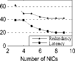
Figure 5. Interface redundancy and multicast latency vs. number of NICs

In Fig.5, we study the impact of the number of NICs on the interface redundancy and multicast latency. We randomly select 60 nodes as the destination nodes and then increase the number of NICs of each node from 3 to 9. The channels are randomly re-assigned to NICs in this process, but we keep the network topology unchanged. When the number of NICs increases, the number of common channels between a node and its neighbors will probably increase, so a node may cover more neighbors with smaller interface redundancy. As a result, the interface redundancy shows a downtrend when the number of NICs increases. When the interface redundancy decreases, fewer NICs are need for a node to transmit a message to its neighboring nodes at a time slot, and more free NICs are available for transmitting other messages at the same time. Therefore, the multicast latency also shows a downtrend when the number of NICs increases. This also explains why our low-latency scheduling algorithm in Section IV is based on the low-redundancy multicast tree built in Section III.

VII.    Conclusion

We consider the multicasting problem in multiinterface multi-channel wireless mesh networks. We indicate that not only the redundancy of forward nodes should be considered in such a scenario, but also the redundancy of the forward NICs should be considered. The concept of interface redundancy is proposed as a new criterion for the multicast redundancy in WMNs, and we prove that building a multicast tree with the minimum interface redundancy is a NP-hard problem. We also propose a heuristics-based greedy algorithm for building a low-redundancy multicast tree. Furthermore, we prove that the minimum-latency multicast scheduling in multiinterface multi-channel WMNs is a NP-hard problem, and present a heuristics-based algorithm for it. Our multicast scheduling algorithm is based on the low-redundancy multicast tree, so the multicast redundancy and latency are jointly reduced in our approach. As a special case of multicast, we also present an approximate algorithm for low-redundancy broadcast in multiinterface multi-channel WMNs, and prove an constant approximation ratio. Finally, the performance of our algorithms is studied under various network conditions and the simulation results showed the effectiveness of our approach.

Acknowledgment

This work was supported in part by Henan Provincial Natural Science Foundation of China under Grant 072300410340 and in part by Foundation of Henan Educational Committee under Grant 2007520062.