Reliability-based design optimization strategy for soil tillage equipment considering soil parameter uncertainty

In the deterministic design optimization [1,2], the designer aims to reduce the engineering design cost without caring about the effects of uncertainties concerning materials, geometry and loading. The resulting optimal solution may therefore represent an inappropriate reliability level. However, the integration of reliability analysis during the optimization process leads to reduce the structural weight in uncritical regions that does not only provide an improved design but also a higher level of confidence in the design. This approach can be carried out in two separate spaces: the physical space and the normalized space. Since many repeated searches are needed in the above two spaces, the computational time for such an optimization is a big problem. The solution of the above nested problems leads to a high computational cost, especially for large-scale structures. The major difficulty lies in the structural reliability evaluation, which is carried out by a special optimization procedure. In order to improve the numerical performance, an efficient method is developed based on the optimality conditions. In this work, we use a statistical study of the soil tillage forces, based on soil property randomness.

Soil Tillage Forces

There are many methods and models had been used to predict the forces acting on the tillage tool. However, the majority of researchers have used the general earth pressure model, proposed by Reece [3]. The total force acting on the tillage tool can be written as follows:

р = P _y+ Pc + Pca + Pq + Pa                                   (1)

Here, P is the total soil cutting force acting on the tillage tool ( kN ), P is the force acting on the tillage tool caused by soil gravity ( kN ), P_c is the force acting on the tillage tool caused by cohesion ( kN ), P_ca is the force acting on the tillage tool caused by adhesion ( kN ), P_q is the force acting on the tillage tool caused by surcharge pressure ( kN ) and P_a is the force acting on the tillage tool caused by tool speed ( kN ). The different force components are given by the following equations:

P7=y. d 2. w. NY

Pc = c. d. w. Nc(3)

Pq = q. d. w. Nq(5)

Pa = Y- v 2d d. w. Na with: у : Soil bulk density (kN/m3), d : Tool working depth (m), c : Soil internal cohesion(kPa), ca : Soil-metal adhesion (kPa), q : Surcharge pressure at the soil surface (kPa), v : Forward tool speed (m/s2), w : Tool width (m), Na : Inertial coefficient (dimensionless), Nca : Adhesion coefficient (dimensionless), Nc : Cohesion coefficient (dimensionless), Nq : Surcharge pressure coefficient (dimensionless), NY : Gravity coefficient (dimensionless)

The coefficients ( N_a , N_ca , N_c , N_q , N _Y ) are defined according to the soil failure model. In this work, we use McKyes and Ali's model [3] to determine these N -factors. We select this model according to its simplicity and accuracy [4]. McKeys and Ali assumed that the soil failure surface from the tool tip to the soil surface was linear, and made an unknown angle P r with the soil surface, Fig. 1. The forward distance of the failure crescent from the blade on the surface was assumed to be equal to the radius r of the crescent.

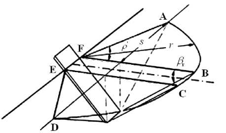
Fig. 1: Proposed soil failure model for narrow blades

The forces acting on the soil segment are illustrated in Fig. 2, including the effects of the density of soil у , the internal friction angle ф , the soil-metal friction angle on the blade surface 5 , the soil cohesion c , the soil-metal adhesion c_a and the surface surcharge pressure q .

Процессы и машины агроинженерных систем

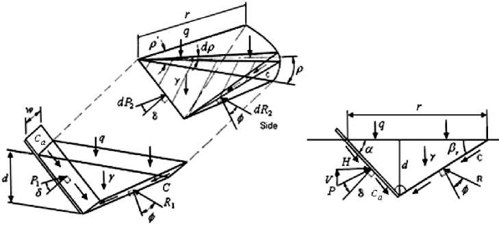
Fig. 2 Forces acting on the soil segment

According to McKeys and Ali's model, Eq. (1) can be written:

1    L   2 5 )

P = [ . Y . r . 1 + .sin ( Р_г+ф )

2     I     3 w J ^V r ⁷

+.

sin (Pr )

5 1,                                     (, ,5 I,1 +— 1 + q.— .sin (pr + ф).| 1 +— 1 +... w) d           I w)

c a [ sin( P _r +ф ) - cot( a ).cos( P _r +ф ) ] + у . v ².

sin (P r +ф)    cos (P r +ф)

cot ( a )      tan ( p _r ) .cot ( a )

]

d . w

sin (a + P r + 5 + ф)

Here, r is the distance from the blade to the forward failure plan ( m ), given by:

r = d . [ cot( a ) + cot( P _r ) ]                                                       (8)

s is the width of the side crescent ( m ), given by:

5 = d .^cot² ( p _r ) + 2. cot( a ).cot( p _r )                                             (9)

a is the Rack angle of the tool from the horizontal (deg), Pr is the angle of the soil failure zone (deg), 5 is the angle of soilmetal friction (deg) and ф is the angle of internal soil friction (deg) . The calculated force in Eq. (7) is a function of the unknown angle Pr. McKyes and Ali obtained this angle Pr by minimizing the dimensionless term of gravity NY. The horizontal force (H) and the vertical one (V) are obtained by combining P with force of adhesion [4] as follows:

H = P .sin( a + 5 ) + c a . d . w .cot( a )                                          (10)

V = P .cos( a + 5 ) - c a . d . w                                              (11)

Structural Reliability

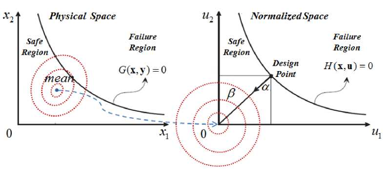
In structural reliability theory many effective techniques have been developed during the last 40 years to estimate the reliability, namely FORM (First Order Reliability Methods), SORM (Second Order Reliability Method) and simulation techniques, see e.g. [5,6]. Here, we consider two kinds of variables: Design variables and Random variables. The image of the random variables in the standard normalized space (Figure 3b) is denoted u , calculated by: u = T ( y ) where T ( y ) is the probabilistic transformation function applied on the physical space (Figure 3a).

138

a )

b )

Fig. 3: a ) Physical spaces, b ) normalized spaces.

For a given failure scenario, the reliability index β is evaluated by solving a constrained minimization problem:

P = min d ( u )    subject to: H ( u ) < 0                                       (12)

with

d   X u2

where u is the vector modulus in the normalized space, measured from the origin see Figure (3). The solution to problem (12) defines the design point P* , see Figure (3b). The resulting minimum distance between the limit state function H ( u ) and the origin, is called the reliability index β.

Reliability-Based Design Optimization (RBDO)

Traditionally, for the reliability-based optimization procedure we use two spaces: the physical space and the normalized space see [7]. Therefore, the reliability-based optimization is performed by nesting the following two problems: Problem I: Optimization problem: this problem seeks to minimize an objective function subject to deterministic constraints and reliability requirements which is defined as follow:

min      f ( x )

subject to g k x <  0       , k = 1,..., K                                          (14)

and      p( x, u )>p t where f(x) is the objective function, gk (x) < 0 are the associated constraints, в (x, u) is the reliability index of the structure, and в t is the target reliability.

Problem II: Reliability analysis: the reliability index β ( x , u ) is the minimum distance between the limit state function H ( u ) and the origin, see Figure 3b. This index is determined by solving the minimization problem:

min        d ( u )

subject to H ( u ) <  0

where d(u) is the distance in the normalized random space, given by d = X ui2 , and H(u) is the performance function (or limit state function) in the normalized space, defined such that H(u) < 0 implies failure, see Figure 3b. In the physical space, the image of H(u) is the limit state function G(y), see Figure 3a [8]. Using the classical approach, the RBDO process is carried out in two spaces, that leads to a high computational time problem. A hybrid approach based on simultaneous solution of the reliability and the optimization problem is developed [9]. This approach consists in minimizing a new form of the objective function F(x,y) subject to a limit state and to deterministic as well as to reliability constraints:

min       F (x, y ) = f (x )■ d p( x, y)

subject to G ( y ) < 0

g k ( x ) > 0         , k = 1,..., K

and        P( x, u )>P t

Процессы и машины агроинженерных систем

Here, d β ( x , y ) is the distance in the hybrid space between the optimum and the design point, d β ( x , y ) = d ( u ). The minimization of the function F ( x , y ) is carried out in the Hybrid Design Space (HDS) of deterministic variables x and random variables y .

Optimum Safety Factor Developments

Formulation Developments

At the MPP, u ^* , is the solution of the Karush–Kuhn–Tucker (KKT) conditions [1] of the FORM optimization problem (1). d H

* u_i

d H d u j

The derivative of the limit state H with respect to u and the derivative of u with respect to the design variable x can be expanded in terms of the original random variables y as follows:

ah a g a Tk-1 (u)       a u * a Tk (u) exx *

--=--k v ’ and = —k^ aui   ayk   aui           axt     ayk ayk

For simplicity, consider now the case of n normalized variables ui , i = 1,...,n, (see Figure 4: two normalized variables u1 and u2). For an assumed failure scenario, we define H(u) < 0 and G(j) < 0 as limit state functions in the normalized space (u-space) and in physical one (y-space). Here, the design point P* can be calculated by min

d² = u² + u 2 + ... + u n

subject to: H ( u 1 , u ₂,..., u_n ) < 0

The Lagrangian function for the problem (19) can be written as

L (u, X, s) = d 2 (u ) + X-[ H (u) + s 2 J

where the inequality constraint in (19) is adjoined by means of the Lagrange multiplier X , after having converted the inequality constraint into the equality H( u ) + s² =0 by introducing the real slack variable s . The optimality conditions for the Lagrangian are:

d L  dd ²   . d H

— =---+ X— = 0  , i = 1, d ut   d ut     d ut

— = H (u) + s2 = 0

5X     v 7

5L

— = 2 s X = 0

8 s

...

, n

The optimality condition for L with respect to s yields the so-called switching condition s X = 0, and the necessary condition d 2 L/ 8 s² >  ⁰ for a minimum of L implies that the Lagrangian multiplier X must be non-negative, i.e., X >  0 . Due to condition (23), we can distinguish between two cases:

Case 1: If the real slack variable is non-zero ( s * 0), the Lagrangian multiplier has to be zero ( X = 0) and the limit state function must be less than zero ( H ( u ) <  0), which corresponds to the case of safety.

Case 2: If the real slack variable is zero ( s =0), the Lagrangian multiplier is non-negative ( X >  0 ) and the limit state is defined by the equality constraint H ( u ) = 0 . The solution here is found on the limit state surface and represents the Design Point .

The first case is not suitable to our reliability-based study whereas the second one is basic for our approach. Using the expression for the square distance d² in equation (19), we get:

Xdh

u, =-       , i = 1,..., n i 2 du i

Problem (17) gives us the reliability index p as the minimum distance between the limit state surface and the origin. This means that the resulting reliability index may be lower or higher than the target reliability index p _t . As we seek to satisfy a required target reliability level for the optimization problem, we can write

n

P ² = 1 u ²

* = 1

To determine X in (24), we now substitute index i by j in (24), square both sides of the equation, and sum from j=1 to n . Using (25), we then obtain

X)2 =-2) n

Pt-______ Г dH f

J = 1 (d u

• j 7

which upon substitution into (24) yields the following expression for the normalized variable u i ,

dH

ui = ±P t

n

duj( 8H

Да u

Equation (27) at the optimum value of the normalized vector can be written in the following form:

ui = ±p t

n

d H

d«J

Г 8H

j Да u

where the sign of ± depends on the sign of the derivative, i.e., dG       *        d G       *

— >  0 О u, >  1 and — <  0 О u _i <  1

S yi                      ^д У,

The calculation of the normalized gradient 8 H I 8 u is not directly accessible because the mechanical analysis is carried out in the physical space rather than in the standard space. However, using theory of statistics we can derive the following expression from which the computation of the normalized gradient can be carried out by applying the chain rule on the physical gradient 8 G I d y :

S H   d G 8 T - ( u )

— =--—    , i — 1,..., n, k — 1,..., K

8 u   cyk   dui where T 1(u) denotes the inverse mapping of u=T(y) from standard normalized space u into the random space y. It is not easy to find the derivative of the inverted probabilistic transformation function T-1(u) with respect to u. Since the calculation of the normalized gradient vector 8H I 8u is not directly accessible and according to our several numerical applications, we find that the normalized gradient in equation (25) considering equation (30) can be expressed as

i — 1,..., n

Equation (27) at the optimum value of the normalized vector can be written in the following form:

^u* = P t

8 G

5 y i

n

Z j=1

d G

5 y j

i — 1,..., n

where the sign of ± depends on the sign of the derivative, i.e.,

8G * 8G *

— >  0 О u, >  1 and — <  0 о u, <  1 , i — 1,..., n ii

Sy i                      ^d y i

Statistical Developments

According to the reliability index definition of Hasofer-Lind [5], an iso-probabilistic transformation can be carried out between the physical space and normalized one (Figure 3). The target reliability index that corresponds to the failure of probability, is numerically computed as follows

P f «Ф ( -р t ) or в t «-ф - ‘ ( P f )                                     (34)

where ф (.) is the standard Gaussian cumulated function given as follows:

Z

^ф ( Z ) = ^= J e ^ 2П -»

² dz ,

Using the basic definition of Hasofer-Lind reliability index (34), we consider a simple normalized mapping transformation for the five most commonly used probabilistic distributions (normal, lognormal, uniform, Gumbel and Weibull distributions).

OSF for normal distribution

In general, when considering the normal distribution law, the transformation between the physical space (or x-Space) and the normalized space (or u-Space) is defined by yi — xi + о iui    , i — 1,..., n(36)

So the design point can be defined as:

yi= f xi,     i =1 ,...,n(37)

Note that using equations (36) and (37), the optimum safety factor associated with u_i ^* can be written as

Sf — 1 + yi.u*, i — 1 ,...,n(38)

where the variance coefficient y _i relating the mean m_i and standard-deviation о _i equals to: у _i — о _i I m, .

OSF for lognormal distribution

For lognormal distribution law, the transformation is defined by y— e ^i+Ziui     , i — 1,..., n(39)

Процессы и машины агроинженерных систем

When considering the lognormal distribution and assuming a single limit state failure scenario G(y) < 0, the equation for the optimum safety factor can be written in a way similar to that presented in section 5.2.1. Hence, we get the optimum safety factors in terms of the optimum values of the normalized variables ui* (see equation (32)), and the equation for the optimum safety factors can be written as

S, = .        exp I / In (1 + y i ) ■ ui I, i = 1,..., n(40)

i                    V)

OSF for uniform distribution

For uniform distribution law, the transformation is defined by yt = a + (b - a )Ф(и1),      i = 1,..., n(41)

and the normalized variables ui are given by u = Ф-11 yi-a |,         i = 1,...,n(42)

V b - a )

where a and b are the end (bound) values of the interval for y t, and Ф is the distribution function. The mean value mt is given by a + b mi = xi = 2 ,        ■ = 1,..., n(43)

and the standard deviation g i by

_ b - a gi = ~^=,      i = 1,..., n(44)

Using equations (18), (34) and (41), we get the following expression for the optimum safety factor corresponding to the optimum value of the normalized variable

u*: Sf = 1 -V3y■ (1 -2Ф(u*)),          i = 1,...,n(45)

OSF for Weibull distribution

For Weibull distribution law, the transformation is defined by yi=v[-In (ф(-и1))] Zk with Ф(-и) = 1 -Ф(и), k: shape factor >0, v : measure factor >0, the mean is given by:

m_; = vГ 1 + — | => v = V k)

m_i rf 1 + ¹

V k and the standard-deviation is given by:

2      2

^g i =^v

rf 1 + ² Vr² f 1 +¹)

V k ) V k )

О Y i =

Г

Г ²

—

№ where Г( a )= J xa-1 e- zdz or a factorial form Г( a ) = ( a -1)! for integers. This way the equation of optimum safety factor can 0

be written as:

S f =   ( ¹ 1 ^ [- ln ( ^{Ф (} - u * ) ) ] ^/k

Г| 1 + ¹ I

V    k )

OSF for Gumbel distribution

For Weibull distribution law, the transformation is defined by yi =v- aln ^- ln (Ф( ui))]

where the mean is given by:

( 0.577 )              ( 0.577

m i = v +1I => v = m i -

V a )            V a and the standard-deviation is given by:

n

n ²

^G i Г— >^a , 2

V6a         6 g i

Using (37) and (52), equation (41a) can be written as

S f , ² = 2 ^ 1 ± 1 - 24 у 2 y ( 0.577 - In [- In ( ф ( « * ) ) ] ) )                                 (53)

Using these safety factors, we can satisfy the required reliability level and significantly reduce the complexity of the problem.

OSF Algorithm

The Optimum Safety Factor (OSF) algorithm can be easily implemented in three principal steps (Fig. 4):

• 1.    Determine the design point: we consider the most active constraint as a limit state function G ( y ). The optimization problem is to minimize the objective function subject to the limit state and the deterministic constraints. The resulting solution is considered as the most probable failure point and is termed the design point.

• 2.    Compute the safety factors: in order to compute these factors using equations (38), (40), (45), (49) and (53), a sensitivity analysis of the limit state function with respect to all variables is required. When the number of the deterministic variables is equal to that of the random ones, there is no need for additional computational cost when the gradient calculation is carried out during the optimization process of the design point. If the number of the deterministic variables is different from that of the random ones, we need only to evaluate the sensitivity of the limit state function with respect to those random variables that are not common with the deterministic.

• 3.    Calculate the optimal solution: in the last step, we include the values of the safety factors in the computation of the values of the design variables and then determine the optimum design of the structure.

  

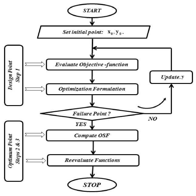
  Fig. 4: Flowchart of OSF approach

  
  

Numerical Application

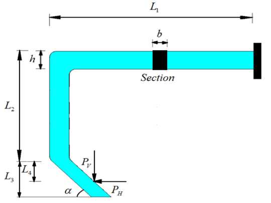
Problem Description

The studied chisel plough illustrated in Fig. 6, can be used primarily to realize the weed control, the seedbed preparation, and other secondary tillage operations. According to the deterministic design studies, the designer proposes a global safety factor on the yield stress value. The RBDO solution can reduce the structural weight in uncritical regions. It does not only provide an improved design but also a higher level of confidence in the design. For example, the allowable stress design methods use a safety factor to compute the allowable stresses in members from the ultimate stress, and a successful design ensures that the stresses caused by the values of the loads do not exceed the allowable stresses c w = c y [Sf where S f is the global safety factor. The values of the proposed safety factors principally depend on the engineering experience that may lead to low reliability level or to high cost. In this application, we consider that the studied parameters are presented by

Процессы и машины агроинженерных систем

probabilistic characteristics. Let us consider that the horizontal and vertical forces follow lognormal distribution laws and theirs probabilistic characteristics are presented in Table 1.

a )

Fig. 5: a ) Schematic drawing of the chisel plough shank with acting forces, b ) Two dimensional optimization problem

b )

Table 1

Probabilistic characteristics of tillage forces

Force Type	Distribution Type	Distribution Parameters	Mean Value	Standard Deviation
P H ( kN )	Lognormal	ц = 0,815 , ^ = 0.421	2,463	1,044
P V ( kN )	Lognormal	ц = - 0,052 , ^ = 0.415	1,032	0,427

The performance criterion, related to the mechanical resistance of tillage machines is determined by the difference between the yield stress and the maximum stress. Therefore, the limit state function that defined the safe region can be written using the following equation:

G(у) = amax-ay ^ 0

Here, x is the vector of deterministic variables and y is the vector of random variables, av is the yield stress and a is the y                           max maximum stress that is given by:

^a max

6 b . h ²

(L2 + L4). Ph +

L4  .PV tan(a)

The limit state function of the simplified shank model, illustrated in Fig. 6, is a function of the following variables as: G (x,y) = f ( P H , P V , a , b , h , L 2 , L ₄). The input geometrical parameters of the studied shank are: L 1 = 600 mm , L₂ = 350 mm ,

L₃ = 150 mm , L ₄ = 75 mm , a = 45°, b = 32 mm and h = 58 mm .

RBDO under Random Loading

Considering given values of the horizontal and vertical forces as: P_H = 2,463( kN ) and P V = 1,032( kN ), the corresponding maximum stress value (using equation (55)) of the initial point equals to: a _max = 63,99( MPa ) . The global safety factor of this point can be calculated by S f = a _y /a max • Using this equation, we get that the global safety factor equals to: S f = 3,67 . Here, we should estimate the reliability level of this structure using equations (12) and (13).

Table 2 Reliability analysis of the studied shank

Parameters	P H ( kN )	P V ( kN )	a max ( MP a )	P	P f
Actual Solution	2,463	1,032	63,99	4,99	3 X 10 - 7
Design Point	8,907	4,560	234,91

Considering two variable problems, the optimization process using ANSYS software (First Order Method) leads to the coordinates of the design point or so-called MPP (Most Probable failure Point) and the actual point (see Table 2). The reliability index of the studied structure equals to: β= 4,99 that corresponds to probability of failure P_f ≈ 3 × 10 ^{- 7}using equation (34). In fact, the nuclear and spatial studies necessitate very small failure probability, the failure probability should be: P_f ∈ [10 ^{- 6} - 10 ^{- 8}] that corresponds to a reliability index β ∈ [4,75 - 5,6] however in structural studies, the failure probability should be: P_f ∈ [10 ^{- 3} - 10 ^{- 5}] that corresponds to a reliability index β ∈ [3 - 4, 25] .

Table 3

RBDO of the studied shank

Parameters	P H ( kN )	P V ( kN )	σ max ( MPa )	β	P f
Optimum Solution	3,420	4,141	100,16	3,00	1 × 10 - 3
Design Point	8,907	4,560	234,91

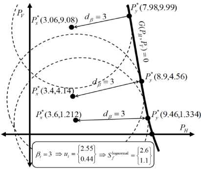
Therefore, we should improve the design reliability to be: β _t = 3 using the recent technology of RBDO based on our OSF developments. Since the loads presented by the horizontal and vertical forces follow the lognormal distribution law, we use equation (40) to compute analytically the optimum safety factors of the loads. Table 3 shows the coordinates of the optimum solution points of the RBDO technology. Figure 7 shows a geometrical description of several solutions. All design points P_y ^* are located on the failure limit state ( G ( P_H , P_V ) = 0) and the optimum solution points P_x ^* are located at the required distance d _β = 3 from the design points.

RBDO under Random Geometry and Loading

Here, we consider the randomness of both geometry and loading parameters. In order to show the influence of different parameters on the maximum stress values, we perform a sensitivity analysis of the maximum stress relative to the geometry and loading. Table 4 defines the sensitivities of the maximum stress with respect to geometry and loading parameters. We note that the derivatives with respect to both parameters L ₁ and L ₃ equal to zeros. Here, we can ignore the influence of these two parameters on the maximum stress values. Therefore, we deal with four geometry parameters ( b , h , L ₂ , L ₄ and α ) and with two loading parameters ( P_H and P_V ).

Table 4

Sensitivity analysis of the maximum stress function

Type	Geometry							Loading
Sensitivity Functions	∂σ max ∂ b	∂σ max ∂ h	∂σ max ∂ L 1	∂σ max ∂ L 2	∂σ max ∂ L 3	∂σ max ∂ L 4	∂σ max ∂α	∂σ max ∂ P H	∂σ max ∂ PV
Sensitivity Values	-1,99	-2,18	0,000	0,137	0,000	0,195	-0,15	0,024	0,0042

Table 5 presents the RBDO results when applying the developed OSF equations for different distribution laws. Table 1 presents the probabilistic data. For both horizontal and vertical forces, the distribution laws (lognormal), the means and the standard-deviations are presented in Table 1 as given data. To compute the OSF, we use equation (40). Since we apply the new strategy on the randomness of the geometry parameters with object of demonstrating its efficiency, the standarddeviations of the random geometry parameters are considered as proportional values of the means ( σ _i = 0,1 m_i ) for simplicity.

Процессы и машины агроинженерных систем

Table 5

Random Parameters	Distribution Laws	OSF Sf i	Normalized Variable u i	Design Point y i	Optimum Solution x i
b ( mm )	Uniform	0,835	-1,958	31,687	37,917
h ( mm )	Uniform	0,835	-2,046	57,673	69,077
L 2 ( mm )	Normal	0,949	0,5133	350,47	332,48
L 4 ( mm )	Weibull	1,303	0,6114	75,174	57,6716
a°	Gumbel	0,879	-0,5366	44,914	51,1
P H ( kN )	Lognormal	1,005	0,2156	9,2501	9,203
PV ( kN )	Lognormal	0,957	0,0895	1,3248	1,383
^ max ( MPa )				234,89	124,73
Volume ( mm 3)				2,01e6	2,83e6
в				3,00
P f				1 x 10 - 3

RBDO of the studied shank under geometry and loading uncertainty

Furthermore, we consider that the length dimension L ₂ , the section shank dimensions ( b and h ), the depth dimension L ₄ and the angle parameter a follow respectively the normal, uniform, Weibull and Gumbel distributions. The sensitivity analysis presented in Table 4 shows that the geometry parameters have a bigger influence than the loading parameters.

Conclusions

In this paper, we develop an efficient methodology that can lead to optimum designs under uncertainties. Here, the developed method controls the structural reliability levels for complex studies. The basic idea of the developed strategy is to find structural sensitivity values with object of determining the influence of each random parameter. An efficient application on the chisel shank plough under the uncertainties on the soil tillage forces is detailed. Here, the tillage forces are calculated in accordance with analytical model of McKyes and Ali. The distributions of soil-tool forces are established to design soil tillage equipments such as shank chisel plough in collaboration with Cranfield University [10]. The advantage of the RBDO using OSF is to define the best compromise between cost and safety. Furthermore, we show that the classical design considering the uncertainty on the loading parameter may not lead to economic or reliable structures.