Remote Sensing Textual Image Classification based on Ensemble Learning

Published Online December 2016 in MECS

Remote sensing image mining or classification is one of the most important methods of extracting land cover information on the Earth [1]. Different from standard alphanumeric mining, image mining or classification is very difficult because images data are unstructured [2]. There are two main image classification techniques, unsupervised image classification and supervised image classification. As for supervised image classification, first, the user selects representative samples called training set for each land cover classes, then a learning classifier is trained by a set of given training data set which contains a lot of training samples, in the end, the trained classifier will be utilized for practical application. In each training samples, there are a low-level feature vector and its related class label. The trained classifier is able to distinguish unknown low-level feature vectors into a class which has been trained. Several classifiers like Maximum Likelihood Classifier, Minimum Distance Classifier has been used for image classification [3].

With the development of remote sensing technology, the spatial and spectral resolution of remote sensing images has been getting higher and higher [4]. It presents new challenges to remote sensing image classification and requires the development of new data classification methods. Many new classification methods such as spectral information divergence, object oriented paradigm appeared [5]. To a certain extent, these classifiers or classification strategy can improve the classification accuracy; however, different classifiers have their own characteristics. For different applications, the performance of classification is not identical [6]. Some of the samples are wrongly classified by one classifier while these samples may be correctly labeled by another classifier, which indicates that there is complementarity between the classifiers. It is difficult to design a powerful model for classifying remote sensing image because the model should not only have main discrimination information of remote sensing image and it should be robust to its variations at the same time.

As a result, only improving traditional methods to achieve robust classification is not always feasible. In 1998, Duin et al. proposed combining multiple classifiers to enhance classification performance of a single classifier [7]. That is, the combination of classifiers is able to amend the errors made by a single classifier on distinct parts of the input space. It is conceivable that the performance of combining multiple classifiers is better than one of the base classifiers used in isolation [8]. The emergence of ensemble learning provides a new research idea for solving the problem of strong correlation and redundancy exists in the bands. Hanson et al. firstly proposed the concept of neural network ensemble [9]. They proved that, the generalization ability of learning systems could be significantly improved through the training of multiple neural networks. In 2011, multiple classifiers ensemble was applied to face recognition [10]. At the same year, support vector machine (SVM) was used as the base classifier to recognize the facial expression [11]. As is known, texture is a vital characteristics for remote sensing image interpretation. However, texture often changes in orientation, scale or other visual appearance thus it is hard to be accurately described by use of a single mathematical model. Generally, several descriptors will utilized for classifying textures, which may improve the classification accuracy and lead to classification difficulty in the meantime.

In the paper, based on the diversity measurement of the base classifiers, J48 classifier, IBk classifier, sequential minimal optimization (SMO) classifier, Naive Bayes classifier and multilayer perceptron (MLP) classifier are selected for ensemble learning. These classifiers respectively use C4.5 classification algorithm, Naive Bayes classification algorithm, k-Nearest Neighbors (k-NN) classification algorithm, artificial neural network (ANN) classification algorithm as the base classifier. In order to evaluate the influence of our proposed method, our approach is compared with the five base classifiers through calculating the average classification accuracy.

The remainder of this paper is organized as follows. Section 2 briefly reviews the ensemble learning. In Section 3, the selection of base classifiers and the proposed method is described in detail. The effectiveness of the proposed method is demonstrated in Section 4 by experiments on several public data sets from UCI machine learning repository and real remote sensing images. Finally, Section 5 draws the conclusion from the experimental results.

• II.    Overview of Ensemble Learning

In a narrow sense, ensemble learning just uses the same type of learners to learn the same problem. For example, we can put all the learners as support vector machine or neural network classifiers. In a broad sense, a variety of learners are applied to solve the problem, which could be also considered as ensemble learning.

The following is the idea of ensemble learning. In general, when learning new examples, the idea of ensemble learning is integrating multiple individual learners and the result is determined by combining the results of multiple learners in order to achieve better performance than a single learner [12]. If considered the single learner as a decision maker, ensemble learning is considered as the decision which is made by a number of decision-makers.

With combining k base classifiers, M , M , , M , an improved composite classification model M ^* is created. A given data set D , D , , D where D (1 ≤ i ≤ k - 1) is devoted to generate classifier M , is used to create k training data sets. The ensemble result is a prediction of class based on votes from the base classifiers. The flow chart of ensemble learning is shown in Fig 1.

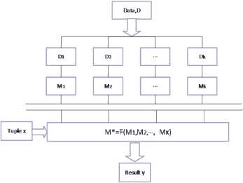
Fig.1. The flow chart of ensemble learning

There are three methods considered in the theoretical guidance to ensemble learning: 1) Sample set reconstruction. 2) Feature level reconstruction. 3) Output variable reconstruction. The way to employ ensemble learning has two steps usually. The first step is to obtain individual models through producing several training subset. The second step is to use the synthesis technology to get the final results on the individual output through the third methods.

Dietterich expounded why an ensemble learner is superior to a single model in three ways [13]. Usually from a statistical perspective, the hypothesis space need to be searched is very large, but it is not enough to accurately learn the target hypothesis as only a few training samples could be used to compare with real samples in the world, which causes the results of learning to be a series of hypotheses that meet the training sets and have approximation accuracy. The hypotheses may well meet the training sets but not hold a good performance in practice, in consequence the choice of only one classify will lead to a big risk. Fortunately, it is able to reduce this risk by considering multiple hypotheses at the same time.

• III.    Multiple Classifiers Ensemble Based on Bagging Algorithm

• A.    Selection of Base Classifiers

  As is discussed above, an important reason for the success of ensemble classifier algorithm is that a group of different base classifiers are employed. Diversity among a team of classifiers is deemed to be a key issue in classifier ensemble [14]. However, measuring diversity is not specific for there is no widely accepted formal definition. In 1989, Littlewood and Miller proposed that diversity has been recognized as a very important characteristic in classifier combination [15]. However, there is no rigid definition of what is directly perceived as dependence, diversity or orthogonality of classifiers. Many measures of the connection between two classifier outputs are able to be derived from the statistical literature, such as the Q statistics and the correlation coefficient. There are formulas, methods and ideas aiming at quantifying diversity when three or more classifiers are concerned, but little is put on a strict or systematic basis due to lack of a definition. The general anticipation is that designing the base classifiers and the combination technology can be helped by diversity measures.

In the paper, we measure the diversity between 5 types of supervised classifier and use the non-pairwise diversity measures, such as entropy, Kappa measure, Kohavia-Wolpert variance, etc.

Let D = { D , D , , D } be a set of base classifiers. Let Ω= { ω , ω , , ω } be a set of class labels, in which x be a vector with n features to be labeled [16].The entropy measure E is defined as Eq.(1)

₁ N ₁

E = min{ l ( x ), L - l ( x )}

N ^∑ j = 1 ( L - [ L /2]) ^{j , j (1)}

E varies between 0 and 1, where E = 0 indicates no difference between base classifies and E = 1 indicates the highest possible diversity. It indicates higher possible diversity when the value of entropy is larger.

Kohavi-Wolpert Variance use a specific classifier model v_x = 1(1 - P ( y = 1| x ) 2 - P ( y = 0| x ) 2 ) to express the diversity of the predicted class label y for x across training samples, where P ( y = ^ | x ) is estimated as an average over different data sets. Averaging over the entire Z , the KW measure of diversity is defined as Eq.(2)

N

KW =     Z ^l ( Z j )( ^L - ^l ( j )

Let p be the average accuracy of each classification, i.e., P = — N^j ’ P NL Z ^

defined Eq.(3)

then Kappa measurement is

_{K = 1}_ £ Z " ! ( x_x L - , ( x ))

N N ( L - 1) P (1 - P )

From Eq.(3), the Kappa value increases with the increase of the correlation between classifiers.

In this paper, J48 classifier, IBk classifier, SMO classifier, Naive Bayes classifier and MLP classifier are selected as the base classifiers. First of all, the five supervised classifiers are introduced briefly. Then, the diversity between these five classifiers is measured by using the non-pairwise diversity measures.

• 1)    J48 Classifier

Decision tree learning construct predictive model as a decision tree, mapping observations about conclusions about an item's target value. Ross Quinlan developed the algorithm of decision tree which called C4.5. C4.5 is an expansion of earlier ID3 algorithm [17]. C4.5 has the same way as ID3 to build decision trees from training data by the concept of information entropy. The method of the construction of decision tree was first derived from Hunt method, which includes two steps [18]. The first step is if there is only one class, the node is a leaf node, otherwise it will enter the next step. The second step is to search for a variable that is to divide the data into two or more subsets of data with higher purity according to the condition of the variable. That is to say, it selects the variable according to local optimality and then returns to the first step. J48 is an open source Java implementation of the C4.5 algorithm in Weka.

The classification rules of the C4.5 algorithm are easy to understand and its accuracy is high. Its main drawback is that it needs to scan and sort the data set repeatedly in the process of constructing the decision tree, which leads to the low efficiency of the algorithm.

• 2)    IBk

The second classification chosen is k -NN. The input of k -NN comprises k closest training sets in the feature space and the output is a class member. An object is classified as a majority of its neighbors, and the object is assigned to the commonest k nearest neighbor. If k = 1 , then the object is assigned to the class of that single nearest neighbor in a nutshell. The training examples, each of which with a class label, are vectors in a multidimensional feature space. In the classification phase, k is a user-defined constant value. The unlabeled vector is classified by attributing the label most frequent among the k training samples nearest to that unknown point. When the training samples are a few, it can simply put the training set as a reference set. When there are many training samples, it can use the existing selection or calculate the prototype of the reference sets. k -NN algorithm has strong adaptability to the tested samples with more overlapping domains.

A commonly used distance metric for continuous variables is Euclidean distance [19]. The length of the line segment connecting points i and j , ( ij ) is the Euclidean distance. In Cartesian coordinates, the distance (d) from i to j , or from j to i when i = ( x _1? x ₂,---, x_in ) and j = ( x _yT, Xj,vxXj_n ) are two points in Euclidean n -space is given by Eq.(4)

d⁽ⁱ , ^j ) = 4 ⁽ X 1 ^- x j 1 ⁾² + ⁽ x 2 ^{- X} j 2 ⁾² + ■ • ■ + ^{( X} n - x jn ^{)2 (4)}

k -NN is a non parametric classification technique [20]. It has higher classification accuracy to unknown and non normal distribution. It has the advantages of intuitive thinking, high feasible degree and clear concept. It directly uses the relationship between the samples, which can reduce the error probability of the classification and avoid unnecessary trouble. Of course, it is a kind of lazy learning method. It has the disadvantages of slow classification speed and strong dependence on sample size.

• 3)    Sequential Minimal Optimization Classifier

SMO is get from the idea of decomposition algorithm to the extreme for solving the optimization problem [21]. It is an iterative algorithm to break the problem into some smallest possible sub-problems, of which the most prominent place is that the optimization problem of two data points can be obtained analytically. Therefore, there is no need to take twice planning optimization algorithm as a part of the algorithm. Each step of SMO selects two elements to optimize [22]. The optimal values of two parameters need to be found and updated the corresponding vectors on the premise that other parameters have been fixed. In spite of more iterations needed to converge, there is an increase in the number of speed because the operation of each iteration is very small.

Based on the principle of structural risk minimization and VC dimension theory of statistical learning theory, Support vector machine (SVM) finds the best balance between the learning ability and the complexity of the model by a certain samples, so as to get the best promotion ability. Compared with the traditional artificial neural network, SVM has the advantages of simple structure. It increases a lot in the generalization performance and solves the local optimum problem which could not be avoided in the neural network. SVM can solve the problems of small collective samples, high dimension and nonlinear. It has a lot of special properties to ensure that the generalization ability in learning period is better. At the same time, it also averts the problem of dimension.

• 4)    Naive Bayes

Naive Bayes classifier is a simple probabilistic classifier based on Bayes' theorem, which has a strong independent assumption [23]. Bayes' theorem is based on the prior probability of a given class known, and then it uses the Bayes formula to calculate the posterior probability. Finally, the class that has the largest posterior probability is selected as the class of object.

In the theory, Naive Bayes is a conditional probability model: suppose the sample space of experiment E to be S , represented by B ,B ,...,B representing n features. A is a event of E and P(A) > 0 . For each of i possible results or classes B , the instance probabilities are P(B,) > 0,(i = 1,2,...,n)  . Using Bayes' theorem, the conditional probability is able to be calculated as Eq.(5)

P ( БД A ) = „ P ⁽ P ^{( B )} , i = 1,2,..., n        (5)

Z P ( A | B j )P ( B j ) j = 1

A clear distinction between Naive Bayes and other learning methods is that it does not explicitly search possible hypothesis space. Naive Bayes algorithm takes less time and considers the logic relatively simple. Naive Bayes algorithm also has a high degree of feasibility and the characteristics of logic and high stability.

• 5)    Multilayer Perceptron

An artificial neural network is a simulation of biological neural network system which are used to evaluate or approximate functions that can depend on a large number of simple computing units connected in some form to form a network [24]. In the stage of network learning, network achieves the correspondence between input samples and correct sample by adjusting the weights. The neural network has a strong ability to identify and classify the input samples, which is to find out the segmentation regions each of which belongs to a class meeting the classification requirements through sample space in fact. A MLP is a feedforward ANN model, which can be regarded as a mapping F : R d ^ R M . What makes a MLP different from other neural network is that a number of neurons use a nonlinear activation function. Learning happens in the perceptron by altering the weight between neurons after each training sample is processed, based on the comparison between the output of the error and the expected results.

Compared with other algorithms, neural network has the advantages of high capacity of noise data, and it has a very good performance for the classification of the training data. Different numbers and types of classifiers are used to measure their diversity. The results are shown in TABLE I.

Table 1. Kappa Measurement of Different Classifiers

number	classifiers	Kappa
2	(J48,IBk)	0.5952
	(J48,SMO)	0.885
	(J48,Bayes)	0.8745
	(J48,MLP)	0.767
	(IBk,SMO)	0.9492
	(IBk,Bayes)	0.8751
	(IBk,MLP)	0.7868
	(SMO,Bayes)	0.885
	(SMO,MLP)	0.7787
	(Bayes,MLP)	0.7768
3	(J48,IBk,SMO)	0.9595
	(J48,IBk,Bayes)	0.9476
	(J48,IBk,MLP)	0.9158
	(J48,SMO,Bayes)	0.9473
	(J48,SMO,MLP)	0.9132
	(J48,Bayes,MLP)	0.9116
	(IBk,SMO,Bayes)	0.9573
	(IBk,SMO,MLP)	0.9232
	(IBk,Bayes,MLP)	0.9149
	(SMO,Bayes,MLP)	0.9143
4	(J48,IBk,SMO,Bayes)	0.9627
	(J48,IBk,SMO,MLP)	0.958
	(J48,IBk,Bayes,MLP)	0.9548
	(J48,SMO,Bayes,MLP)	0.9542
	(IBk,SMO,Bayes,MLP)	0.9572
5	(J48,SMO,MLP,IBk,Bayes)	0.9671

It can be seen from TABLE I, if we choose two classifiers from all classifiers, the best choice are IBk classifier and SMO classifier. Similarly, if we choose three classifiers from all classifiers, the best choices are J48 classifier, IBk classifier and SMO classifier. If we choose four classifiers from all classifiers, the best choices are J48 classifier, IBk classifier, SMO classifier and Bayes classifier. If we want to get better results, we need to choose the five classifiers. Therefore, J48 classifier, IBk classifier, SMO classifier, Naive Bayes classifier and MLP classifier are chosen to conduct ensemble learning.

• B.    Multiple Classifiers Ensemble based on Bagging Algorithm

  Bagging algorithm is a kind of ensemble learning method improving the classification by combining classifications with randomly selecting training sets, which proposed by Breiman in 1994 [25]. If there is a training set of size m , it is practicable to draw m random instances from it with replacement. The m instances are able to be learned, and this process can be duplicated several times. Some duplicates and omissions are contained in the instance compared to the initial training set, since the draw is with replacement. Through the process, each cycle results in a classifier. According to the construction of several classifiers, the forecast of each classifier will be a vote to influence the final forecast.

Algorithm: Bagging algorithm

Input:

• 1.    D = {( x i ;y i ),( X 2 ; y 2 ),...,( X m , y m )} , a set of m training tuples;

• 2.    T , the number of models in the ensemble;

• 3.    L , a classification learning scheme (J48, IBk, SMO, Naive Bayes and MLP).

• 4.    Output: The ensemble --- a composite model,

• 5.   Method:

• 6.   for t = 1 to T do

• 7.    create bootstrap sample, D_t = Bootstrap ( D ) , by sampling D with replacement;

• 8.     use D and the learning scheme L to derive a model,

• 9.    endfor

• 10.    To use the ensemble to classify a tuple, X :

• 11.    Let each of the T models classify X and return the majority vote;

T

H(X) = arg max У l(У = ht (X)) . When the value yeY in the parentheses is a true proposition, the sum is 1. Otherwise, the sum is 0.

h _t ;

Given a training set D = {( X 1 ; y 1 ),( x 2 ; y 2 ),...,( X m , y m )} of size m , bagging algorithm generates T new training sets D_t , each of size m' , by sampling from D congruously. For each sample set, the probability is 1 - (1 - 1/ m ) ^m . For large m , the unique examples will be 1 - 1/ e = 63.2% and the rest will be duplicates .

The T models are fitted using the above T kinds of samples which known as a bootstrap sample and combined by casting votes. It has the correct classification rate r = [maxP(■ | X)Px (X) . Based on iX bagging algorithm, the probability of correct classification can be as Eq.(6)

r A = l Cmax ^{P (} i । ^X ) ^P X ^{( X} ) ⁺ L ^[ У I^{( Ф} А ^{( X} ) = ¹ )P ^{( 1} । ^{X )] P} X ^{( X} )

^{X x} i                             ■                                  (6)

It can be seen from the correct rate that the result of bagging algorithm is better than the results obtained by a single prediction function.

• IV. Simulation Results and Discussion

• A.    Experiments for Public Data Sets

  In order to evaluate the performance of multiple classifiers ensemble based on bagging algorithm, five public data sets from UCI machine learning repository named “Image segment”, “german_credit”, “hepatitis”, “ionosphere” and “soybean” are used in this part. For example, “Image segmentation” data set has 19 continuous attributes, 210 training samples and 2100 test samples. It was randomly selected instances from a database of 7 outdoor images and each instance is a 3x3 region. The images were segmented to create a classification for each pixel. The classes of the “Image segmentation” data set are brickface, cement, foliage, sky, path, window and grass. The general information of other data sets, such as the number of instances, the number of attributes and the number of classes are shown in TABLE II.

Table 2. General Information of Public Data Sets From UCI

Data Sets	Instance	Attribute	Class
segment	2310	19	7
german_credi t	1000	20	2
hepatitis	155	19	2
ionosphere	351	34	2
soybean	683	35	19

Before calculating the classification accuracy, some approaches are chosen to data cleaning as a process. It not only ensures the degree of uniformity and accuracy of the data set, but also makes the data set more conducive to the implementation of the mining process by changing the internal structure and content of the data file. The data preprocessing not only improves the quality of the data sample set but also improves the quality of the data mining algorithm and reduces the running time.

For neural network backpropagation algorithm, normalization helps speed up the learning phase after normalizing the input values for each attribute. If using a distance-based method, normalization can help prevent attributes with originally large ranges from overweighting attributes with originally smaller ranges. Considering the classifiers chosen, we use min-max normalization to preprocess the data. In the attributes of Image segmentation data set, the values of region-centroid-col, region-centroid-row, region-pixel-count, short-line- density-5, short-line-density-2, vedge-mean, vegde-sd, hedge-mean, hedge-sd, intensity-mean, rawred-mean, rawblue-mean, rawgreen-mean, exred-mean, exbluemean, exgreen-mean, value-mean, saturatoin-mean and hue-mean are [1,254], [11,251], [9,9], [0,0.333], [0,0.222], [0,29.222], [0,991.718], [0,44.722], [0,1386.33], [0,143.444], [0,137.111], [0,150.889], [0,142.556], [-49.667,9.889],[-12.444,82],[33.889,24.667], [0,150.889], [0,1], [-3.044,2.912], respectively. It is clear that the 19 numeric attributes are not in the same range, so they need to be unified to a certain extent.

The experiments use Normalize , which is an unsupervised filter in Weka. By min-max normalization, suppose that min and max are the minimum and maximum values of an attribute, A . The value v ′ is mapped by the value v of A in the range [0 ， 1] by minmax normalization, computing as Eq.(7)

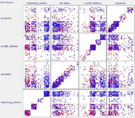
Fig.3. Visualization of the german_credit data set using a scatter-plot matrix with part of attributes

v - min v'=           A max - min

Fig.2, Fig, 3, Fig, 4, Fig.5 and Fig. 6 are the visualization of the above five data sets using a scatterplot matrix.

Plot Matrix                age                 SEX               STEROID           ANTIVIRALS

«Ик"	° a      °®,’° ^ «	« #	®
“«к	‘V gg	о ®	Ш в ^
«®V » > к о °: °	«	® о 8 ®	Ш ^ M ‘ -
	'5 1	4 x	i

Fig.4. Visualization of the hepatitis data set using a scatter-plot matrix with part of attributes

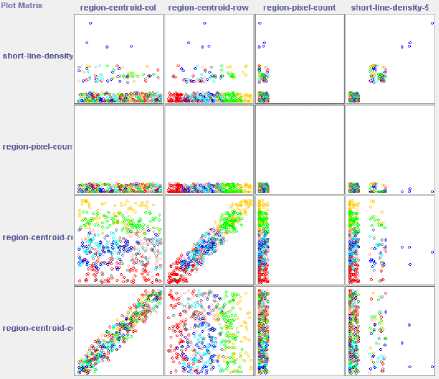
Fig.2. Visualization of the Image Segmentation data set with part of attributes

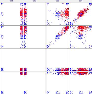
Fig.5. Visualization of the ionosphere data set using a scatter-plot matrix with part of attributes

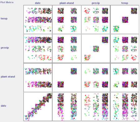
Fig.6. Visualization of the soybean data set using a scatter-plot matrix with part of attributes

In the experiment, C4.5 algorithm, k -NN algorithm, SVM algorithm, Naive Bayes algorithm, ANN algorithm and ensemble learning algorithm are used to classify the test data sets separately. For five public datasets, TABLE III shows average classification accuracy of using the J48 classifier, IBk classifier, SMO classifier, Naive Bayes classifier, MLP classifier and bagging classifier.

Table 3. Comparison Of Classification Accuracy For Five Public Data Sets

Data Sets	J48	IBk	SM O	Naiv e Baye s	MLP	Bagging
segment	96.9%	97.1%	93.0 %	80.2%	96.2%	97.7%
german_ credit	70.5%	72%	75.1 %	75.6%	72%	76.4%
hepatitis	83.8%	80.6%	85.1 %	84.5%	80%	85.8%
ionosphere	91.4%	86.3%	88.6 %	82.6%	91.1%	92.0%
soybean	91.5%	91.2%	93.8 %	92.9%	93.4%	94.4%

It can be seen from TABLE III, for “Image segment” data set, the average classification accuracy of IBk classifier is significantly higher than the other four kinds of base classifiers, reaching 97.1%; as for “german_credit” data set, the average classification accuracy of Naive Bayes reaches 75.6%; for “hepatitis” data set and “soybean” data set, the average classification accuracy of SMO classifier is higher than the other four kinds of base classifiers, reaching 85.1% and 93.8% respectively; in the experiment of “ionosphere“ data set, the average classification accuracy of J48 classifier reaches 91.4%, however the average classification accuracy of IBk algorithm, SMO algorithm, Naive Bayes algorithm and MLP algorithm are 86.3%, 88.6%, 82.6%, 91.1%, respectively.

It can be seen that, for different data sets, the results of the classification accuracy are different, because the performance of the base classifiers are different. There is no one kind of classifier has absolute advantage. This is also the purpose of this experiment. Based on the difference and information complementarity between the base classifiers, it combines different classifiers with bagging algorithm and gives full play to the advantages of each base classifier. From the experimental data of TABLE III, the average classification accuracy of ensemble learning algorithm based on the above five kinds of classifiers is higher than the average classification accuracy using one of the base classifiers separately. It can be seen that the results of the five data sets using bagging algorithms for classification respectively are 97.2%, 76.1%, 85.8%, 92.0%, 94.7%.

• B.    Experiments for Remote Sensing Image Data Sets

In order to further illustrate the performance of our method on real remote sensing images, we selected some real remote sensing images as training data. There are 684 instances which are divided into four classes, including resident, paddy field water and vegetation area. Some training samples of each class are shown in Fig.7, Fig.8, Fig.9 and Fig.10.

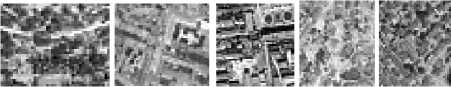
Fig.7. Resident training samples

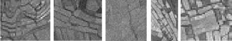
Fig.8. Paddy field training samples

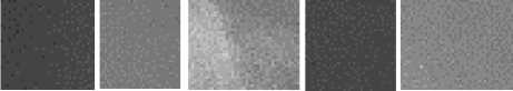
Fig.9. Water training sample.

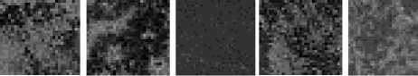
Fig.10. Vegetation training samples

The same as five public data sets, remote sensing image data set uses min-max normalization to deal with the original data of 22 attributes, including variance, skewness, prominence, energy, absolute value and texture energy of each order. Fig.11 shows visualization of the remote sensing image data set using a scatter-plot matrix.

Then C4.5 algorithm, k -NN algorithm, SVM algorithm, Naive Bayes algorithm, ANN algorithm and ensemble learning algorithm are used to classify remote sensing image data set separately. Table IV shows average classification accuracy of using the J48 classifier, IBk classifier, SMO classifier, Naive Bayes classifier, MLP classifier and bagging classifier for remote sensing image data set.

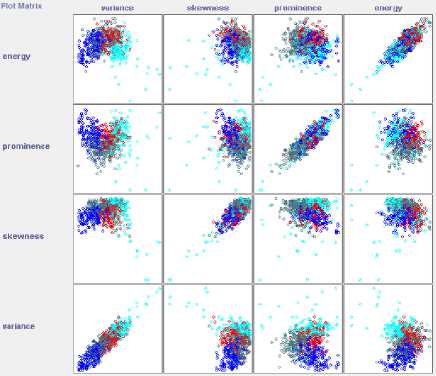
Fig.11. Visualization of the remote sensing image data set using a scatter-plot matrix with part of attributes

Table 4. Comparison of Classification Accuracy for Remote Sensing Image Data Set

Data Sets	J48	IBk	SMO	Naive Bayes	MLP	Bagging
Remote Sensing Image	81.2%	78.6%	86.5%	85.1%	86.9%	89.1%

From TABLE IV, the average classification accuracy of using the J48 classifier, IBk classifier, SMO classifier, Naive Bayes classifier, MLP classifier and bagging classifier for remote sensing image data set are 81.2%, 78.6%, 86.5%, 85.1%, 86.9%, successively. As for the result of bagging algorithm, it rises to 89.1%, which is nearly 2% higher than MLP, which performs best as a single classifier in base classifiers. It may be deduced that as for texture images classification, ensemble learning is a promising approach which could acquire the satisfied results in practice.

• V. Conclusion

In order to improve the classification accuracy of remote sensing image, our method uses ensemble learning to combine the classifiers of J48, IBk, sequential minimal optimization, Naive Bayes and multilayer perceptron, which classify the data sets by straight voting. At last, five set of public data and real remote sensing images are selected to verify the results. The experimental results show that multiple classifier ensemble can effectively improve the classification accuracy of textural remote sensing images. However, in the paper, classifiers are integrated with the sample mode, in the future, some better way would be employed .

Acknowledgment

This work is funded by the National Natural Science Foundation of China under Grant No.41301371 and funded by State Key Laboratory of Geo-Information Engineering, No. SKLGIE2014-M-3-3.