Removal of image blurring and mix noises using gaussian mixture and variation models

The field of digital image processing alludes to the use of computer algorithms to extract helpful data from digital images [1-4]. The whole procedure of image processing may be divided into three prime stages:

• 1)    Image acquisition:  Converting 3-D visual

information into 2-D digital form appropriate for storage, processing and transmission.

• 2)    Processing: Enhancing quality of an image by enhancement, restoration, etc.

• 3)    Analysis: Drawing out image features; quantifying shapes and then recognition.

In image acquisition stage, input is an actual 3-D scene while output is a corresponding digital image. On the other hand, both input and output are digital images at second stage of processing, where the output is an enhanced form of the input. In the last stage, input is still a digital image but the output is description of its contents. Fig. 1 illustrates a block diagram.

Image Acquisition

Format Conversion

De-noising/ De- blurring etc.

Analysis Feature Extraction/ Pattern Recognition etc.

Output Image

Input Image

Fig.1. Image processing and noise filtering

• A.    Noise

Noise in an image is the irregular variation of color or brightness of the image created by the sensor and circuitry of a scanner or digital camera [5-13]. Image noise is taken as an unwanted by-product of captured image. The sorts of noises are as given below:

• 1)    Gaussian noise (Amplifier noise): The standard model of amplifier noise is additive. Gaussian noise is independent at every pixel and also independent of the signal intensity.

• 2)    Salt-and-pepper noise: An image comprising salt-and-pepper noise consists of dark pixels in bright regions and bright pixels in dark regions.

• 3)    Speckle noise: Speckle noise is a granular noise that inherently exists and corrupts the quality RADAR images. SAR is produced by unified processing of backscattered signals from numerous distributed targets.

• B.    Gaussian Blur

Gaussian Blur is that pixel weights aren't equal and they decrease from kernel center to edges. The effect of Gaussian Blur is a filter which de-focuses an image. The blurring is dense in the center while at the edge is feathers [12-13].

Frequently, digital cameras have very little noise in their pictures. Here we will illustrate an approach to dispose of that noise by making use of the selective Gaussian blur filter [14-16]. The fundamental idea behind specific Gaussian blur is that the photo areas with contrast below a certain threshold get blurred.

The composition of paper is as follows: In section II, various restoration filters are discussed. In Related Work Gauss-Total Variation model (G-TV model) is presented in section III. In section IV, Gaussian Mixture-Total Variation Model (GM-TV model) is presented. In section V of the paper simulation results are discussed. Finally, section VI of the paper concludes the work.

distributed (i.i.d.) as a Gaussian distribution N(0, a2) , i.e.,

g ^{( x} ) = ^{( k} * f ^{)( x} ) ⁺ " ^{( x} )          (5)

II. Various Image Restoration Filters

Restoration of image or Denoising is the method of getting the original image from the corrupted image given the knowledge of the degrading factors [12-17]. It is utilized to evacuate noise from the degraded image without affecting and maintaining the edges with other details.

P ( ^{( k} * f ^{)( x} )^— g ^{( x} )/ ^{a 2}) = ~j= ^exP^—- 42na²

L ( f , ^{a 2}) = ⁿ x _en -r= ^exp^{— 2}

4 2.na

|( k * f )( x )— g ( x )|2 , 2a²        '

| ( k * f )( x ) — g ( x )|2

^          2 a ²          ’

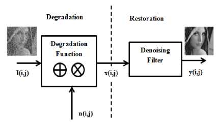
Fig.2. Image Degradation and Restoration process

Minimizing log-likelihood function

E , (.f - a ² ) = j J

n

_x I^{( k} * f ^{)( x} ) ^— g ^{( x} )|²

+ —j in a ² dx

2 П V 7

► dx

where a is an unknown constant.

Minimizing the above equation is equivalent to minimizing the residual [19,20]

In Fig. 2, image degradation and restoration process is shown. O(i, j) is an input object n(i, j) is degrading term (may include noise, blurring or both) so x(i, j) is x (i, j) = O (i, j) + n(i, j)

or

x(i,j) = о(i,j)x "(i,j)

y (i, j) = H [ x (i, j)]

H is filter operator.

In simplified form, да y (t) = j x(t)h(t — т)dT(4)

—да where x(t) is input image, h(t) is filter impulse function and y(t) is the output image.

• III.    Gauss-Total Variation Model (G-TV Model)

A new interpretation of the ROF model is developed in this section that is based on statistical approaches. In the following, we consider that the noise intensity n ( x ) or ( k * f )( x ) + n ( x ) is a random variable and all these random variables are independent and identically-

1 I k * ^{f —} g |£2

The minimization problem defined above is ill-posed, hence we incorporate a regularization term and gets the following cost functional [17-18]

E (f ,a2) = E1( f, a2) + ^J (f)

Considering TV regularization term as

J (f) = J^Vf |2 + pdx

n

v(_f a if Jl^{( k} * ^{f )( x} )^— g ^{( x} )2L

Ei(f, a) = 2‘ I--------- I

• 2 n I

+ — J in ( a ² ) dx + X J ^| V f |² + в dx

2 nn

Algorithm:

Choose initial values of f 0 and (a2) . For different values of n = 1,2,3,4,...... soon

• 1.    Evaluate f" ⁺¹ , under the condition

• 2.    Evaluate ( ст ²) " +1 , under the condition

• 3.    Check for the convergence, if converges STOP, else go to STEP 1.

fn+1 = arg min E (f ,(a2)")

( ст ²) " ⁺¹ = arg min E ( f " ⁺¹ ,( ст ² ))

Check for the convergence, if converges STOP, else go to STEP 1.

(0)"+1 = arg min E(f"+1,(0))

In step 2, it is noticeable that parameters of mixed pdf need to be evaluated. For minimization, we modify function as

IV. Gaussian Mixture-Total Variation Model (GM-TV Model)

Assume at each point X gQ , the intensity of noise "  ( x ) or ( k * f )( x ) — g ( x ) is a random variable and all the random variables { " ( x ) | x g Q } are independent and identically-distributed with the following probability density function [19]:

M

E1( f,0)=2 EJ

² I = 1 q

M

+1EJ

² l = 1 q

M

⁽ к * f ^{)( x} ) ^— g ⁽ x ) ^— м 2

2 ст 2

> to " ( x ) dx

M l=1

M

E j a dx

where each p is a Gaussian density function with mean 2

M l and variance CT_Z , and the parameter set 0 = { a ₁,..., a _M , ^ 1 ,..., M m , ст^ ,..., ст М } is chosen such that

M

Ea=1

l =1

Where

ton (x) = to, (x |( k . f") (x) — g (x), 0" )

V =1

After adding variation parameter we get,

In other words, the probability density function (PDF) is a mixture of M individual Gaussian components with different ratios.

^M E 1 ( f . ®)=2 EJ ² I = 1 q

I^{( k} * ^{f )( x} ) ^— g ^{( x} ) ^— Mi^

2 ст ,²

to n ( x ) dx

^E 1 ( ^{f , 0}) =j- ^ln E ^a exp

Q        i = 1 ^CT i

I^{( k} * ^f )( x )^- g ⁽ x )^- n1\ л--Z----------------- ?

2 ст,ст

dx (15)

MM

i = 1 q

¹ = 1 Q          q

J ( f ) = J _P ( f ) = J ^ V f |² + в dx    ⁽¹⁶⁾

q

The above is to be minimized under the M constraints E al = 1 . Thus the problem is very much l =1

similar to the Gauss model except a new constraint.

Algorithm 1:

1. Evaluate f " ⁺¹ , under the condition

Algorithm 2:

Choose initial values, f 0 , 0° and calculate to^ (x ) .

For different values of "  = 1,2,3,.....

Find f"+1, such that f"+1 — f"   3     Vf"       Mk (k * f" — g—Ml))«"

^A t       Mv f ^ p+ e I ¹ =        ^{( ст} )”

fn+1 = argmin E (f ,(0)")

2. Evaluate ( ® ) " ⁺1 , under the condition

Find, 0" ⁺¹ and to " ^{+ 1} such that

a n ⁺¹ = —j a ( x ) dx       (21)

A -

A = J 1 dx              (22)

-

J l⁽ k * f^{n + 1 )( x} ) ^- g ^{( x} )l ^a n ^dx a n ^{+ 1} = ----------r------------------   (23)

J a dx

-

( ^ )"⁺1

J |( k . Г ⁺¹)( x ) - g ( x ) - a l ⁺¹( = -_____________________

a ⁺¹ ( x ) =

adx j adx -

• p, ( k * f n ⁺¹ )( x ) - g ( x )| a ⁺> , ²) n ⁺¹

M                                          ()

E a n ⁺¹ P v ^{( k} * ^{fn +1 )( x} ) ^- g ^{( x} ) | a n ⁺¹ , ⁽ a 2 ) n ⁺¹

v = 1

a ," ⁺¹

p = (( k * f n ⁺¹)( x ) - g ( x )| a ⁺¹,( ^ 2) n ⁺¹)

^pi = 1     , „ ^exP^-

V 2n to ²) ^{n +1}

' I ( k * f n ⁺¹)( x ) - g ( x ) - al ⁺¹[ )⁽²⁶⁾

2(^2) n ⁺¹

This is known as Gaussian Mixture-Total Variation equation. The key point in this model is the introduction of a ( x ) which lies between 0 and 1. For each

M point x € — , E a (x) = 1 . The M = 1 values of i=1

a ( x ) can be thought as weighing average of M deblurring components. Here, if M = 1 , this model is equivalent to Gauss model.

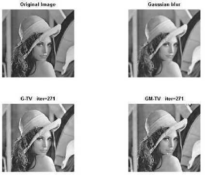
Fig.3. (a) Original image (b) Gaussian blur with variance 1 (c) G-TV iteration 271 (d) GM-TV iteration 271

The obtained PSNR and SSIM from G-TV model are 44 dB and 0.912 and from GM-TV model obtained PSNR and SSIM, are 44 dB and 0.92. Thus the performance of the GM-TV model is superior to G-TV model in case of de-blurring of images.

In Fig. 4, estimated pdfs are shown. As noise is not present therefore a vertical line is observed. However, due to blurring pixels values change slightly, thus a smaller broadening is observed in estimated pdf. The broadening in estimated pdf using GM-TV model is lesser in comparison to G-TV model.

1 0 -1 -2 -3

-6,

-----InPDF of salt-and-pepper noise

• ♦ Eestimated InPDF by G-TV model                                   ~

  ---Eastimated InPDF by GM-TV model

43.8     -0.6     -0.4     -0.2      0      0.2     0.4     0.6     0.8      1

• V.    Results

In this section, simulation results for both Gauss and Gaussian Mixture model are presented. In Fig. 3, Lenna image is shown which is made blur using Gaussian blur with variance 1. However, no noise is added to the original image. Thus, these results can be thought of as de-blurring results. The recovered images using G-TV and GM-TV are shown in Fig. 3(c) and (d) respectively. It is found that the image is well recovered after 271 iterations. Moreover, the quality of the recovered image is good.

Fig.4. Estimated PDF by both the models (var=1)

In Fig. 5, Lenna image is shown which is made blur using Gaussian blur with variance 9. The recovered images using G-TV and GM-TV are shown in Fig. 5(c) and (d). It is found that images are well recovered after 441 iterations. Moreover, the quality of the recovered image is again good. But the performance of GM-TV model is much better. Thus as the blurring increases more number of iterations are required to recover the image. The obtained PSNR and SSIM from G-TV model are 29.8 dB and 0.65 and from GM-TV model obtained PSNR and SSIM are 39.2 and 0.80. Thus the performance of the GM-TV model is much superior to G-TV model in case of de-blurring of images.

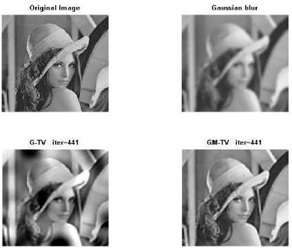
Fig.5. Original image (b) Gaussian blur with variance 9 (c) G-TV iteration 441 (d) GM-TV iteration 441

In Fig. 6, estimated pdfs are shown. As noise is not present therefore a vertical line is observed. However, due to moderate blurring pixels value changes, thus a broadening is observed in estimated pdf. The broadening in estimated pdf using GM-TV model is lesser in comparison to G-TV model. It can be inferred from the figure that as the variance increases the obtained pdf broadening in G-TV model is more. Thus, G-TV model is more susceptible to blurring in comparison to GM-TV model.

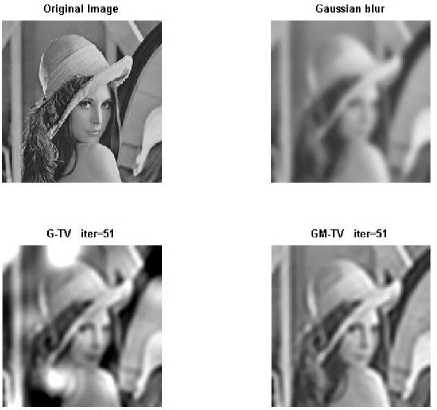
Fig.7. (a) Original image (b) Gaussian blur with variance 25 (c) G-TV iteration 441 (d) GM-TV iteration

In Fig. 8, estimated pdfs are shown. As noise is not present therefore a vertical line is again observed. However, due to high blurring pixels value changes significantly, thus a larger broadening is observed in estimated pdf. The broadening in estimated pdf using GM-TV model is lesser in comparison to G-TV model. From Fig .4, 6 and 8, it can be observed that estimated pdf from GM-TV model remains nearly same while for G-TV model it broadens as blurring increases.

A

3 -

2 -

О -

-2 -

-3 ■

----InPDF of salt-and-pepper noise

♦ Eastimated InPDF by G-TV model ---Eastimated InPDF by GM-TV model

-0.8     -0.6     -0.4     -0.2       0

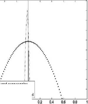
Fig.6. Estimated PDF by both the models (var=9)

---InPDF of salt-and-pepper noise

• Eastimated InPDF by G-TV model

---Eastimated InPDF by GM-TV model                    \ o's * 0.6 0.4    0'2 О 0.2    0.4    06 o# 1

In Fig. 7, Lenna image is shown which is made blurred using Gaussian blur with variance 25. The recovered images using G-TV and GM-TV are shown. It is found that images are not well recovered after 51 iterations. As we increase the number of iterations due to the over fitting of Gaussian model recovered image becomes black. Therefore is case of heavily blurred image quality of recovered image is not good. The obtained PSNR and SSIM from G-TV model are 12.28 dB and 0.54 and from GM-TV model obtained PSNR and SSIM are 13.05 dB and 0.66.

Fig.8. Estimated PDF by both the models (var=25)

In Fig. 9, PSNR (dB) vs. sigma is plotted in the form of BAR graph. It is clear from the figure that as the variance increases, the value of PSNR decreases.

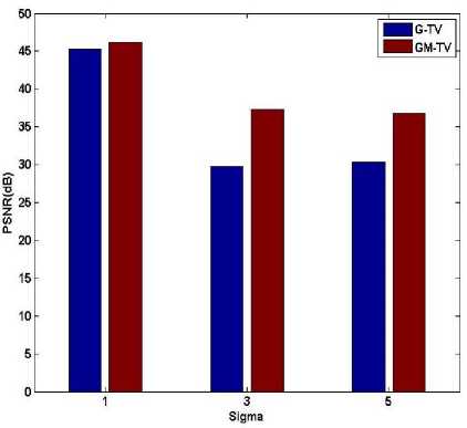
Fig.9. PSNR (dB) vs. Sigma (blur only)

Similarly, SSIM vs. sigma is plotted in Fig. 10. Here SSIM decreases for both the methods as sigma increases. However for sigma 3 and 5, PSNR is nearly same (Fig. 9), in fact it is more for sigma 3. Thus, PSNR cannot be considered as good quality measure.

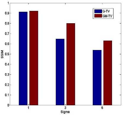
Fig.10 SSIM vs. Sigma (blur only)

In Fig. 11, only Gaussian blurring is considered with mean 25 and variance 1. Thus, due to the lesser variance blurring is less. In Fig. 11, the Gaussian blurred image is very much similar to the original Lenna image however as noise is introduced, the blurred and noisy image is not clearly visible. The recovered images using G-TV and GM-TV are shown, and it is clear that the recovery of the image is better in case of GM-TV model. Still recovered images are not of good quality especially under G-TV model.

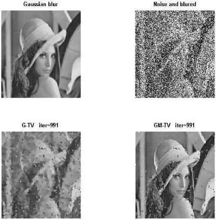
Fig.11. (a) Gaussian blur (b) Gaussian and salt and pepper noise with variance 1 (c) G-TV iteration 991 (d) GM-TV iteration 991

In Fig. 12, obtained pdfs for G-TV and GM-TV are shown. Now due to presence of salt and pepper noise a random pdf which is somewhat similar about vertical axis is shown. In presence of noise estimated pdf by G-TV model is broader in comparison to earlier case of blur. A major change is observed in GM-TV model pdfs, it is very broad now.

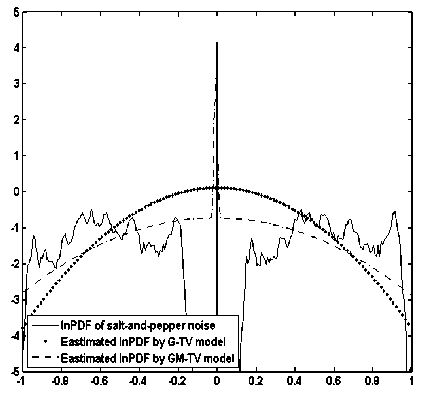
Fig.12 Estimated PDF by both the models in presence of noise (var=1)

In Fig. 13, only Gaussian blurring is considered with mean 25 and variance 9. Thus due to lesser variance, blurring is less. The recovered images using G-TV and GM-TV are shown, and it is clear that the recovery of image is better in case of GM-TV model. Still recovered image under G-TV model is of poor quality. Now due to larger blurring, pixel expansion is much and GM-TV model is now able to distinguish between blur and noise, thus results improve.

Fig.13. (a) Gaussian blur (b) Gaussian and salt and pepper noise with variance 9 (c) G-TV iteration 1991 (d) GM-TV iteration 1991

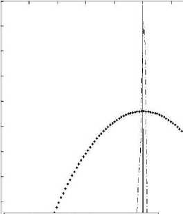
In Fig. 14, obtained pdfs for G-TV and GM-TV are shown. Now due to presence of salt and pepper noise, a random pdf which is somewhat similar about vertical axis is shown. In presence of noise estimated pdf by G-TV model is broader in comparison to earlier case of blur. A major change is observed in GM-TV model pdfs, it is very broad now. However, with increase in variance no significant changes are observed in the graphs.

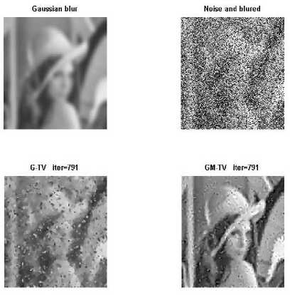
Fig.15. (a) Gaussian blur (b) Gaussian and salt and pepper noise with variance 25 (c) G-TV iteration 791 (d) GM-TV iteration 791

In Fig. 16, obtained pdfs for G-TV and GM-TV are shown. Now due to presence of salt and pepper noise a random pdf which is somewhat similar about vertical axis is shown. In presence of noise estimated pdf by G-TV model is broader in comparison to earlier case of blur. A major change is observed in GM-TV model pdfs, it is very broad now. However, with increase in variance no significant changes are observed in the graphs (Fig. 14 and Fig. 16).

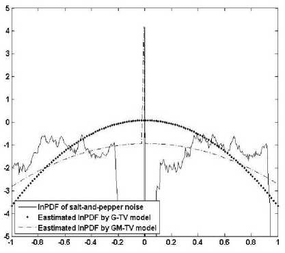
Fig.14. Estimated PDF by both the models in presence of noise (var=9)

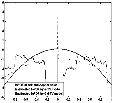
Fig.16. Estimated PDF by both the models in presence of noise (var=25)

In Fig. 15, only Gaussian blurring is considered with mean 25 and variance 25. Thus due to the lesser variance blurring is less. The recovered images using G-TV and GM-TV are shown, and it is clear that the recovery of image is better in case of GM-TV model. Still recovered image under G-TV model is of poor quality. Although the performance of GM-TV is not good, yet it is better than G-TV model.

In Fig. 17, PSNR (dB) vs. sigma is plotted in the form of BAR graph. It is clear from the figure that as the variance increases the value of PSNR decreases. However for sigma 1 the PSNR (dB) for G-TV model is 32.7 while for GM-TV it is 37.6. For sigma equals 3 and 5, PSNR for G-TV is 31.2 and 31.8 respectively. For GM-TV for sigma 3 and 5, PSNR for GM-TV is 38.4 and 34.3 respectively. Thus obtained values clearly suggest that GM-TV model is much more superior to G-TV model.

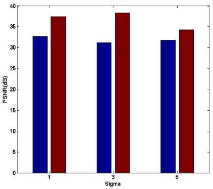
Fig.17. PSNR (dB) vs. Sigma (Blur and noise)

Similarly, SSIM vs. sigma is plotted in Fig. 18. Here SSIM decreases for both the methods as sigma increases. However for sigma 1 the SSIM for G-TV model is 0.558 while for GM-TV it is 0.802. For sigma equals 3 and 5, SSIM for G-TV is 0.524 and 0.323 respectively. For GM-TV for sigma 3 and 5, SSIM for GM-TV is 0.8 and 0.507 respectively. Thus obtained values clearly suggest that GM-TV model is much more superior to G-TV model.

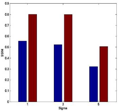
Fig.18. SSIM vs. Sigma (Blur and noise)

• VI.    Conclusions

In this paper, two methods are detailed which are capable of removing blurring and noises in digital images.

On the basis of obtained results, following conclusions can be made:

• •    G-TV model is quite effective in reconstructing images with blur and uniform distributed noise without changing the regularization parameter λ directly.

• •    However, it still could not work well when the image is contaminated with blur and mixed noise.

• •    Moreover, with lesser Gaussian blur variance, image recovered in lesser iterations.

• •    However, as the variance increases, number of

iterations required to recover images also increases.

• •    G-TV model fails to remove noise; however, it

performs well for de-blurring of the image.

• •   GM-TV model works well even on noisy images.

• •    GM-TV model is also capable of removing both

blurring and noise in the images.