Research of the semi-Markovian process in conditions of limitedly rare changes in its state

In this work the SM-process has been considered [1]; it is the general flow of flow models with homogeneous events.

We shall give a definition of the Semi-Markovian (SM) process. For this purpose we have considered a twodimensional homogeneous Markovian stochastic process {£ ( n ), т ( n )} with a discrete time. Here £ ( n ) the ercodic Markov chain with a discrete time and matrix P = [ p νk ] accept the probabilities of transition for one step [2]; the process т( n ) accepts non-negative values from the continuous set.

Then we determine the Markovian transition function F ( v , x , k , y ) for the process {^( n ), т( n )}:

F ( k , x ; v, y ) =

= P{^(n +1) = k, t(n +1) < x|£(n) = v,t(n) = y}.

We shall consider two-dimensional processes such as {£ ( n ), т ( n )} for which the following equalities are correct:

F (v, x; k, y) = F (v, x; k), that is F(ν, x, k, y) does not depend on the values of the y process т(n).

Denote

F (к, x; v) = Avk (x) =

= P{^(n +1) = k, t(n +1) < x| £(n) = v}.

Matrix A ( x ) with elements A_νk ( x ) can be called Semi-Markovian.

The stochastic process of homogeneous events:

t1 < t2 < - < tn < tn+1 < - is called the Semi-Markovian process or SM, set by matrix A(x); if for moments tn the approaching of its events is correct, the following equations are performed:

t n + 1 = t n ^+T( n ⁺ 1 ) .

In view of (1), thee transitive probability matrix of Markov’s chain £ ( n ) is defined by equation:

P = A (^).

This chain for the Semi-Markovian process is called the embedded Markov chain.

In general case, the elements of the Semi-Markovian matrix have a place in the multiplicative form which can be written as:

Avk (x) = P{^(n +1) = k,t(n +1)< x| ^(n) = v} =

= P{t(n +1) < x,|^(n) = v,£(n +1) = k}x

X P {^( n + 1) = k, |^( n ) = v} = Gvk ( x ) Pvk , where Gνk (x) – is the conditional distribution function of an interval length of the Semi-Markovian process in condition that at the beginning of this interval the embedded Markov chain has an accepted value ν, and at the end of it will accept value k.

Note, due to equation:

A v k ( x ) = G V k ( x ) P V k ,                ⁽²⁾

matrix A ( x ) can be written as a Hadamard produce:

A ( x ) = G ( x ) * P                (3)

of two matrixes G ( x ) and P , and it is possible to suppose, that the Semi-Markovian process is set by two matrixes G ( x ) and P .

The state of the semi-markovian process at the moment of time t n < t ≤ t n+ 1 is called state k of its embedded Markov chain, accepted at the beginning of interval ( t n , t n + 1 ].

The research of the Semi-Markovian process will be will carried out in conditions of limit rare changes of (LRCS) flow conditions; i. e. the transition from one state of the embedded Markov chain to another is realized extremely rarely.

The conditions of limit rare condition changes of the Semi-Markovian process are formalized by the following equation for matrix P (δ) transition probabilities of its embedded Markov chain:

P ( 5 ) = I + 5- Q ,                   (4)

where δ – is some small parameter (δ → 0); I – is an identity diagonal matrix.

Matrix Q with elements q νk is similar to a matrix with infinitesimal characteristics and has the same properties: k ≠ ν matrix elements q νk > 0, and also is correct:

E q v k = 0, E q v k =- q kk . k             k *v

The Semi-Markovian matrix for the SM process in condition of LRCS:

• 1.    k = v

• 2.    k + v

A_kk ( x ,5 ) = P { ^ ( n +1 ) = k , t ( n +1 ) <  x £ ( n ) = k } =

= G kk ( x ){ 1 ⁺⁵ - q kk } .

A v k ( x ,5 ) = P { ^ ( n +1 ) = k , t ( n +1 ) < x |^ ( n ) = v } =

= G v k ( ^x H- q v k .

On the other hand, in the multiplicate notation (3) of the Semi-Markovian matrix let’s substitute (4) and get:

A ( x ,5 ) = G ( x ) * { I + 5- Q } .             (5)

Let’s state m ( t ) – as the event number of the Semi-Markovian process, which appeares during t on the interval [0, t ).

The process m ( t ) is non-Markovian, therefore it is necessary to make it Markovian by a method of additional variables. Let’s define the process: z ( t ) – is the length of an interval from time moment t till the moment of approach for the next event in the considered SM-process.

However, the two-dimensional process {m(t), z(t)} is not Markovian, therefore let’s consider one more stochastic process s(t) with piecewise constant continuous realizations on the left, defined by equation:

^S ( t ) = ^ ( n + 1 ) , if t n <  t <  t n + 1 .

This is on the interval ( t n , t n+ 1 ] process, s ( t ) accepts and assures that value of the embedded Markov chain ξ( n ) accepts the beginning of the following interval [1].

The three-dimensional stochastic process is thus defined as { s ( t ), m ( t ), z ( t )} with two additional variables s ( t ) and z ( t ) – is Markovian with continuous time and with probability distribution:

P ( s , m , z , t , 5 ) = P { s ( t ) = s , m ( t ) = m , z ( t ) <  z } , (6)

it is simple to create a system of differential Kolmogorov equations:

dP ( s , m, z, t, 5) dP ( s , m, z, t, 5) dP ( s , m ,0, t, 5) ----------- =--- dt

dz dP (v, m -1,0, t, 5)

d z

X

+ E v=1

d z

A vk ^{( z} ) ,

at the set initial conditions:

P ( s ,0, z ,0,5 ) = R ( s , z , 5 ) ,

P ( s , m , z ,0,5 ) = 0, m > 1,

+

where function R ( s , z , δ) – is the stationary distribution of the two-dimensional Markovian process { s ( t ), z ( t )}.

Let’s denote the function:

X

H ( s , u , z , t , 5) = S e j^um P ( S , m , z , t , 5),        (9)

m = 0

where j = V-1 - is an imaginary unit.

For these functions it is possible to write down the following Cauchy problem from system (7) and initial condition (8):

d H ( s , u , z , t , 5 )    d H ( s , u , z , t , 5 ) d H ( s , u ,0, t , 5 )

d t      "      d z             d z

+ e, £5H (v,u,0,t,5)Avk (z,5) , v=1        dz

H ( s , u , z ,0, 5 ) = R ( s , z , 5 ) .

Let’s denote:

H ( u , z , t , 5 ) = { H ( 1, u , z , t , 5 ) , H ( 2, u , z , t , 5 ) ,... } , also matrix A ( z , δ) with elements A kν ( z , δ), then from (10) we receive the following:

d H ( u , z , t , 5 )    d H ( u , z , t , 5 ) d H ( u ,0, t , 5 )

• a t             a ^{z     +}     a z     ^x

• { e ju A ( z , 5 ) - 1 } ,                                    (11)

H (u, z ,0,5) = R (z, 5), where I – is an identity matrix, and vector R (z, δ), is defining the initial condition of problem (11) with components R (s, z, δ), as shown in [3], given by:

R(z,5) = к1 (5)r j(P(5)-A(x,5))dx, where r – is the stationary value probability distribution of the embedded Markov chain ξ(n); magnitude κ1(δ) – is defined by equation:

к (5) = ^7KF, rA (5) E where matrix A(δ) is defined by equation:

to

A ( 5 ) = j ( P ( 5 ) - A ( x , 5 ) ) dx .

Asymptotic probability distribution of event numbers, the arrival of which is in the SM-process in time t is found in a condition of limit rare changes for the conditions of process.

Let’s denote:

lim H ( u , z , t , 5 ) = H ( u , z , t ) .

5^01 V                  \ Z

In problem (11), considering (12) we shall execute a limiting transition at δ → 0, then H ( u , z , t ) we will receive in the set of an independent Cauchy problems [3; 4]:

d H ( u , z , t ) d H ( u , z , t ) d t           d z

H (u, z ,0) = R (z), dH(u,0,tV . a

' , , ) { euA ( z ) — I } , d z     ¹             ’ (13)

where:

lim P ( 5 ) = I , lim A ( z , 5 ) = A ( z ) , lim A ( 5 ) = A , 8^0 ^v '       5^0 ^{v 7 v} ' 5^0 ^v '

lim к. ( 5 ) = к. , lim R ( z , 5 ) = R ( z ) .

5^0       ^{7      1}     5^0 ^{v 7 v 7}

Considering the kind of matrix A ( z ), from (12) are we get a set of independent differential equations:

d H ( s , u , z , t )    d H ( s , u , z , t ) d H ( s , u ,0, t )

dt             dz            dz(14)

x{ ejuGss (z)-1}, the initial conditions are given in the following way:

H (s, u, z ,0) = R (s, z).(15)

The solution of a problem (14–15) by applying of the transformation of Fourier–Stieltjes:

to

ф( s, u, a, t) = j ej “z dzH (s, u, z, t).(16)

The function φ ( s , u , α, t ) is satisfied by the following equation:

and the initial condition:

ф( s, u, a,0) = j ej “zdzH (s, u, z ,0) = to

= j ej “z dzR (s, z) = R * (s, a), where to

G * s ( a ) = j .d z G ss ( z ) .

The solution of the differential equation (17) is:

и e-j“t /т?‘ Г5 aH ^j“T dH(s,u,0,t) x ф i s, u, a, t j — e л .zv i s, a j ~ i ex v                         \ vd

(               0.

x| e^juG * _s ( a ) - 1 | d tI .

As lim ф( s, u, a, t t ^to V

to

) = j ej “zdzH (s, u, z, *) — 0, that, having directed t to infinity in equation (19) we get:

0 — R * ( s , a ) + j e^{j aT д} H ^ s | ^{j ,0}L ^т ) ( e^juG * _s ( a ) - 1 ) d t .

From this equality we find the Fourier transformation dH (s, u ,0, t) in τ from function:

dz j ejaT dH(s, u,0, t) dt = R. (s, “) (1 - euGss (“)) 1 . 0>

Having executed the reverse Fourier transformation we identify:

^d H ⁽ s , u ^{,0, T)} = — f e-^{j aT} R * ( s , a ) (1 - e^juG ; ( a )F * d a .

dz       2n J V ЛV Л

-to

Equation (19) considering the received transformation will be:

ф ( s , u , a , t ) = e ^{j a} t <  R *

t

( s , a ) + j e^

— x

2 n

to x j e-jytR•(s,y)(1 -ejuG*s(y)f dy(eJjG*ss(a)-1)dtI . (20)

-to

Knowing, that H ( s , u , ∞, t ) = H ( s , u , t ) = φ ( s , u , 0, t ), R ^* ( s , 0) = κ₁ r_sA_ss , G ^* _ss (0) = 1, we get an expression for function H ( s , u , t ):

H ( s , u , t ) = к , r s A ss + J je -^{jy t} d t R * ( s , y ) x ^{2 n}--to 0                          (21)

x ( 1 - e^juG * s ( y ) )^{- 1} dy ( e^j - 1 ) .

дф ( s , u , a , t )                         d H ( s , u ,0, t )

— -------- = - j “ф( s, u, a, t)+-----------x d t               v ’        dz

Considering:

x { ., G ( a ) - 1 } ,

j e -^{jy t} d t =

— ( 1 - e - jyt jy

),

and:

R •( 5, y ) = J ejydzR (5, z ) = r jyK r(G(y)- 1)

= ^K 1 ^r5 j e j ^d J ( 1 - ^G55 ( x ) ) ^d x = ----—------- .

00            jy

We shall denote the equation (21) as:

r

H ⁽ 5, u, t) = ^K1 rA + -^ J — ( ^{1 -} e - j ^yt ) ^x

^{2 n} -L У                  (22)

x ( 1 - G ( y ) )( 1 - eC ( y , , dy ( e j - 1 ) .

Let’s denote h ( u , t ) = 2 H ( 5 , u , t ) as:

s

(eju -1)K h (u, t) = 2 H (5, u, t) = 1 +x

2 n

Г- x J -2(1 -ej )2r (1 -G„ (y))(1 -e-G, (y)) dy.

-„ y

Knowing, that h ( u , t ) = 2 H ( 5 , u , t ) ® 2 H ( 5 , u , t , 8 ) = ss

r

= 2 e jn P ( n , t ), and sorting it to the right part of the n =0

received equation of the exponent levels e^ju , it is possible to write down the following asymptotic equation as:

^r                     ( e ju - 1 ) k.

h(u, t) » 2 ejumP(m, t) = 1 + 2x m=0

rr xJ -2-(1 -ej)2r (1 -G* (y))2ejX" (y)dy =

-r У              5m

r

=1 ’S J 7(1"e-" >2r (1 - c* (y)dy+ n-r y5

r

+ -^ J -2 ( 1 - e -j^yt ) 2 r_s ( 1 - G 55 ( y ) ) 2 e jXr ^-1 ( y ) dy .

2n -r y             5m

Then the asymptotic probabilities distribution of possibility P 1 ( m , t ), number of events m which start in the SM time process t , look the following way:

r 1

P1(°'t) =1 -K- J ;2i1 -e-" )2 r. (1 -G'- (y)dy• 2n-r y r 1

IP!(m• t)=5;J-.(1 -e-")2r.(1 -c;,(y))'x

.          -r y x2 e-c;;--1 (,.) dy, m=1

where

P₁ ( m , t ) ® P ( m , t ) .

Above were obtained formulas that allow us to find the asymptotic probability distribution of the number of events, which happen in the SМ-process in time t. This distribution was also found in prelimit situations [1], by using methods of integrated transformation. It is necessary to find out how close the results received by the asymptotic method of analysis are to the results received in prelimit situations. For this purpose there is a magnitude A = max

n

Л

F ( " , t ) - F ( n , t )

Л

, where F ( n , t ) - is

the function of distribution, obtained from the asymptotic analysis; F ( n, t ) – is the function of distribution for prelimit situations, received in [1].

Let:

f- 3 1

Q = ^ 3   - 4

[ 4    2

	' 1	- e	5 x	1     -2 x 1 - e
c ( x ) = ^	1	- e	-4 x	1 - e - x
	1	- e	6 x	1 - e - 3 x

² . ,

- 6

-10 x

1 - e

1 - e "9 ^x

1 - e "8 ^x

t = 6.

From table it can be seen that at the given parameters of values the magnitude A are:

Deviation results of the asymptotic from prelimited analysis

δ	0,001	0,0005	0,0001	0,00005	0,00001
A	0,0427	0,0216	0,0042	0,0021	0,0003

On fig. 1–3 are the probability distributions of the number of events in the SM-process, which occurred in time t = 6, obtained by using the asymptotic analysis and the prelimit situation.

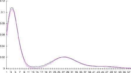
Fig. 1. Distribution probabilities of a number of events for the SM-flow at δ = 0,001

0.12 0.1 0.08 0.06 0.04 0.02
0 1	3 5 7 9 111315171921232527293133353739414345474951535557

Fig. 2. Distribution probabilities of a number of events for the SM-flow at δ = 0,0001

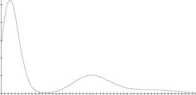
1 3 5 7 9 11 1315 1719212325272931333537 3941 4345474951 5355 57

Fig. 3. Distribution probabilities of a number of events for the SM-flow at δ = 0,00001

In this research we have found the distribution of the asymptotic probability for a number of events occurring in the SM-flow in time t. By reducing the parameters δ, the deviation results of the asymptotic analysis for the prelimited varies: at δ ≤ 0,0001 it is equal to less than 1 %. Also, it is necessary to notice, that the obtained distribution is multimodal.