Research on Fuzzy Enhancement in the Diagnosis of Liver Tumor from B-mode Ultrasound Images

Liver cancer is one of the most popular malignant tumors in Asia. In patients with chronic viral infection, the severity of the disease may be ranked from asymptomatic healthy carriers to patients with cirrhosis of the liver[1-3]. The gold standard for diagnosis of patients with diffuse parenchyma liver diseases depends primarily on a needle biopsy of the liver. However, the pathological measurement of diseases such as hepatitis and liver cirrhosis may be severely biased due to the sampling error in the biopsy specimen. B-mode ultrasound diagnosis is the first option in popular diagnostics due to its economy, efficiency, noninvasiveness. Affected by the quality of ultrasound images of liver cancer, benign expression of malignant tumors and observer’s visual fatigue, careless mistakes, and diagnostic level, not all liver cancers can be detected accurately. Thus, it’s necessary to provide the medical operators a computer aided diagnosis (CAD) system which is helpful to reduce the possibility of wrong diagnosis or missed diagnosis[4-6].

According to the ultrasound image representation of hepatocellular carcinoma (HCC) and echo type in the tumors, there are five types of primary carcinoma of liver, which are corresponding to low echo type, equal echo type, high echo type, mixed echo type and diffuse type respectively. Most CAD systems are based on texture features which are extracted from the B mode ultrasound images. These features are used to classify three sets of ultrasonic liver images-normal liver, hepatoma, and cirrhosis. Texture features include the spatial gray-level dependence matrices, the Fourier power spectrum, the gray-level difference statistics, and the Laws’ texture energy measures [7-9]. Classifiers include Bayes classifier, K means, neural network[6,10], support vector machine (SVM)[11,12], et al. However, the accuracy of classification is greatly affected by quality of the ultrasound images. Ultrasound images quality are greatly effected by the ultrasound machine settings and the operation of operators which directly affect the classification accuracy.

In this paper, we aim to use fuzzy enhancement to preprocess the input ultrasound images in order to decrease the effect resulted from different ultrasound machine settings in the computer aided diagnosis of liver cancer from ultrasound images. According to the characteristic of B-mode ultrasonic liver image, we will compare the classification accuracy of different classifiers with the fuzzy enhancement [13,14] used in processing of images. The classifiers in this paper include K-means, back-propagation neural network, SVM.

• II.    METHODS

The object of enhancement technique is to process a given image so that the result is more robust than the original for classification of liver cancer. The methods so far developed for image enhancement may be categorized in two broad classes, namely, frequency-domain methods and spatial-domain methods. The technique in the first category is based on modifying the Fourier transform of an image, whereas in spatial domain methods the direct manipulation of the pixel is adopted. The technique used here is based on the modification of pixels in the fuzzy property plane of an image. The property domain is extracted from the spatial domain using fuzzifiers which play the role of creating different amounts of fuzzification in the plane. The fuzzy operator, contrast intensification, is taken as a tool for enhancement.

• A.    Fuzzy feature plane

Define Ω={X} is a set , µ _D ( x ) is a function of each element in Ω where 0 ≤ µ _D ( x ) ≤ 1. µ _D ( x ) is used describe the subjection of X to D. D is a fuzzy set of Ω and µ _D ( x ) is subjection function of D. According to the concept of fuzzy subset, a M×N image X with L grey

levels can be considered as a fuzzy points set , denoted as , ■ Р11/ Г! p12 /x12 L  P1N / x1 N " X = P21/ x21 p22 /x22 L p1N/x1N (1) _Pm 1/xM 1 pM2/xM2 • K pMN / xMN _ operation above,

than 0.5. We can use transformation T ₁ to denote the

M d ^{( x} ) = T 1 ⁽ M d ^{( x} )) =

| T ^¹⁾( M d ( x )) (0 <  M d ( x ) <  0.5) [ T ⁽²⁾( M d ( x ))(0.5 <  M d ( x ) <  1)

or

= UU p_tJ/ x -      ( i = 1,2,..., M ; j = 1,2,..., N )        (2)

Where p_ij describe the state that the pixel ( i , j ) has the feature P ij (0 <  P j <  1). P j is called fuzzy feature. If the comparative grey level of the pixel is considered as the interest fuzzy feature, and x_ij is the grey level of pixel ( i , j ), X _max is the maximum grey level in the image, the fuzzy feature can be explained as follows, P = F(X j ) = [1 + ( x max — j ^     ( = 1,2,..., M j = 1,2,..., N)     (3)

F p

Where Fp is fuzzy parameter. Eq 3 shows that when x„ ^ X™, P, ^ 1 ; when x. decreases , ij max ij                             ij

P_ij decreases correspondingly. Therefore, fuzzy feature P_ij denotes the possibility that the pixel ( i , j ) has the maximum grey level. The plane composed by all P j , ( i = 1,2,..., M ; j = 1,2,..., N ) is called fuzzy feature plane. when X - = 0 , p j is a finite positive number,

P j = [1 + ( ,    '    ¹                  (4)

F p

The range of P j is [ a ,1].

• B.    Model of fuzzy enhancement

If the contrast enhancement operator CEO which is applied on the fuzzy set D can produce a new fuzzy set CEO ( D ) = D , its subjection function is expressed as:

\ 2[ M d ( X )]²      (0 <  M d ( x ) <  0.5)

M d ^{( x} ) M ceod ^{( X} )  1                2 _m , ,    , ,

[ 1 — 2[1 — m _d ( x )] ⁽ 0.5 <  M d ^{( x} ) < ¹⁾ (5)

This operation decreases the fuzzification of fuzzy set D, and increases the value of m _d ( x ) when it is more than 0.5, decreases the value of m _d ( x ) when it is less

When the Eq 6 is applied on the fuzzy feature plane, then

P j ( x ) = T k ( P j ) =

_Tk (1)_{( Pij )}

T k ⁽²⁾( P ij )

(0 <  P j < 0.5) (0.5 <  P j < 1)

Where T_k can be regarded as the iterations of T1. when k ^» , T_k ( P j ) will produce a binary image. If T_k is iterated with finite times, the image can be enhanced obviously. The detailed of fuzzy enhancement algorithm in this paper can be described as,

• (1)    Extract the fuzzy feature of image, and constitute the fuzzy feature plane : P j = F ( x j ).

• (2)    On the fuzzy feature plane, use contrast enhancement transformation T_k to enhance fuzzy feature P_ij and obtain the fuzzy enhanced P_ij ^' .

• (3)    Apply inverse transformation on the new fuzzy feature plane to get the enhanced output images x - = F ^' Pi/) .

Considering P ij e [ a , 1] , plane P ij possibly contains the region where P j is less than a . all the value of P j is replace as a when P j is less than a , its corresponding constraint condition is denoted as a <  P j <  1 , which is the constraint condition of inverse transformation. In the process of fuzzy enhancement, suitable fuzzy parameter F_P is important to the enhancement result, which is related to critical point X_c in the image space, X_c should satisfy the following conditions:

xy > Xc , Pj> 0.5 , xy < Xc, Pj< 0.5.                   (8)

We can change the enhancement result through adjusting the fuzzy parameter F _P . In our application , critical point X_c is empirically less than the half of the average grey level of the image.

• III.    EXPERIMENTAL METHODS

The experimental procedure is described as the Fig 1. The subimage including region of interest (ROI) was extracted manually from the acquired liver ultrasound images firstly. Then fuzzy enhancement was applied to improve the subimage quality. Texture features were extracted to train and test the classifiers.

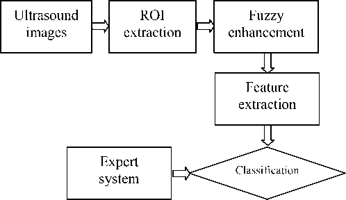
Fig.1 The flow chart of the processing

• A.    Image acquisition

A total of 256 sonograms from patients, including 60 liver cancers (malignant (MAL)), 30 hemangioma (HEM) and 166 normal liver tissue(NOR), which were divided into two groups. 30 liver cancer images, 31 hemangioma images and 83 normal liver images were used as training dataset, and the rest are used for testing.

• B.    Determination of ROI

To reduce the impact of translation of the focal region, a focal region in the liver cancer image were selected manually by physicians since the size of focal region in different images are different. For example, the tumor in low echo liver cancer images is always small, but in high echo liver cancer images is large. This should cause the size of our region of interest (ROI) became variable. The size of each image is 90*93 with 256 gray levels in our experiments. The effect of size of the regions to the classification accuracy was reported in our previous experiments[2]. The size of region is empirically determined as 30*30 pixels larger than the usual size of liver tumor in this study.

• C.    Feature extraction method

ultrasound images[15]. These features are regarded as the input of the classifiers.

• (1)    FOS

The first order statistical features employed in this research were as follows:

• 1)    Mean:    µ = ∑ ^{L - 1} iP ( i )

i = 0

• 2)    Standard deviation:     σ ² = ∑ ^{L - 1}( i - µ )² P ( i )

i = 0

1 L - 1

• 3)    Skewness: s = ₃ ∑ ( i - µ )³ P ( i ) σ ³ i = 0

1 L - 1

• 4)    Kurtosis: K = ₄ ∑ ( i - µ )⁴ P ( i ) σ ⁴ i = 0

• 5)    Energy : ENERGY = ∑ ^{L - 1}[ P ( i )]²

i = 0

• 6)    Entropy : ENT = - ∑ ^{L - 1} P ( i ) log[ P ( i )]

i = 0

• (2)    GLCM

• 1)    Moment of inertia:

• ASM = ∑∑ m h ² k hk

• 2)    Energy:

CON = ∑∑ ( h - k ) ² m hk hk

• 3)    Entropy:

ENT =-∑∑mhklogmhk hk

• 4)    Correlation coefficient:

∑ ∑hkmhk - µxµy

COR = ^hk

σxσy mhk is the appearing frequency of pairs of pixels, which has grey level of h and k respectively. µx,µy,σx,σy分別 are the mean and standard deviation of mh and mk respectively, here, mk= ∑mhk mh= ∑ mhk.

• (3)    GLRLM           ^{h           k}

• 1)    Short run emphasis:

  In order to validate the method, we used the original ultrasound images and fuzzy enhancement processed images to do the experiments. 25 features from first order statistic (FOS), gray-level co-occurrence matrix (GLCM), gray-level run-length matrix (GLRLM) and Gray level difference matrix (GLDM) were extracted from the

  
  

  SRE =

  
  

  N_g N_{l ∑∑ (} m gl

  
  

  ^g

  
  

  g = 1 l = 1

  
  

  l ²

  
  

  N g N l ∑∑ m gl g = 1 l = 1

  
  

  )

  
  

  2) Long run emphasis:

  N g

  
  

  N l

  
  

XX (12 mg-)

^LRE = g^--

XX mg- g=1 l =1

• 3)    Gray level nonuniformity:

N g N l

X (X mg- )2

^GLN = g^—

XX mg- g=1 I=1

• 4)    Run length nonuniformity:

N l ^Ng

X (X mg- )2

^RLN =    ---

XX m g-g = 1 l = 1

• 5)    Run percentage:

directions, five texture features were obtained:

1) Contrast: con = X i ² f ( i 1 6 )

• 2)    Mean: mn = X if ( i | 6 )

• 3)    Entropy: ent = - X f ( i 1 6 )log f ( i 1 6 )

• 4)    Inverse difference moment:

v- f ( i 1 6 ) idm = > —;---

^^ i ² +1

• 5)    Angular second moment:

asm = X [ f ( i 1 6 )]²

• (5 ) LAWS

Laws developed the texture energy features using the following 1D kernels: L=[1,6,15,20,15,6,1], E=[-1,-4,-5,0,5,4,1], S=[-1,-2,1,4,1,-2,-1], W=[-1,0,3, 0,-3,0,1], R=[1,-2,-1,4,-1,-2,1], O=[-1,6,-15,20, -15,6,-1], where, L, E, S, W, R, and O denote level, edge, spot, wave, ripple, and oscillation, respectively. The texture energies from the following kernels are typically computed. Using these 1D kernels of length seven, 2D convolution kernels are generated by convolving a vertical 1D kernel with a horizontal 1D kernel. Five texture features were obtained.

N_l N g

XXm.

RP = J=Lg Z 1--

P

(4) Grey level dependant matrix (GLDM)

We consider here a class of local properties based on absolute differences between the gray levels of pixels in the ROI. Let I(x,y) be the image intensity function. For any given displacement 6 = (Ax, Ay) , let 15 (x, y) =| I(x, y) -1(x + Ax, y + Ay) |, and f (i |6) be the probability density of I6 (x, y). The value of f (i 16) is obtained from the number of times I6 (x, y) occurs for a given 6 , i.e. f (i | 6) = P(I6(x,y) = i). If a texture is directional, the degree of spread of the values in f (i | 6) should vary with the direction of 6 , given that its magnitude is in the proper range. Thus, texture directionality can be analyzed by comparing spread measures of f (i | 6) for various directions of 6 . In the present study, four possible forms of the vector 6 were considered: (0,d), (d, 0), (-d, d), and (-d, -d), with d being the interpixel distance, each of which corresponds to a displacement in vertical, horizontal, 135º and 45 º direction, respectively. From each of the density functions corresponding to one of the above-mentioned

(a)

(c)

(e)

(b)

(d)

(f)

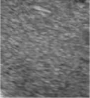
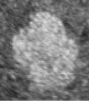
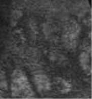
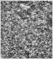
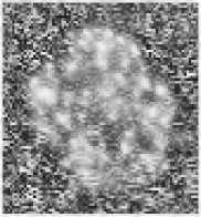
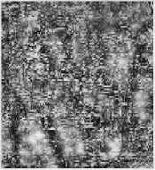
Figure. 1 Results of fuzzy enhancement

• IV.    RESULTS

In our experiments, three classifiers including K means, back propagation (BP) neural network (NN), support vector machine (SVM) were compared so as to evaluate the influence of fuzzy enhancement on the different classifiers.

• A.    Experimental result of fuzzy enhancement

One of results of fuzzy enhancement are shown in Figure.1. The left columns are original images. (a) is normal liver tissue image, (c) is hemangioma image and (e) is liver cancer image. The right columns in Figure 1 are their corresponding images processed by fuzzy enhancement.

• B.    K means experimental results

Table.1 Classification result of liver cancer from normal liver tissue with K means.

	Original images	Fuzzy enhancement processed images
sensitivity	50%(15/30)	56.67%(17/30)
1 - specificity	69.39%(68/98)	75.51%(74/98)

Table.2 Classification result of liver cancer from hemangioma and normal liver tissue with K means.

	Original images	Fuzzy enhancement processed images
sensitivity	60%(18/30)	73.33%(22/30)
1 - specificity	78.31%(65/83)	87.95%(73/83)

Normal liver 56.02%(93/166 )    57.83% ( 96/166 )

Hemangioma 40% ( 12/30 )     36.67% ( 11/30 )

• B.    BP neural network experimental results

We did the same experiments as K means using BP NN[17]. The target error we defined in our BP neural network is 0.01. With this target error our NN method can get the best classification accuracy in our experiments. However, if the value of target error is too small, the convergence rate is slow and it is easy to result in overtraining. If the error is too big, the approximation is not accurate. Table 4 and Table 5 show the classification results of differentiating liver cancer from normal liver tissue and liver cancer from abnormal liver respectively. Three classes result with BP NN is shown in Table 6. The results demonstrate that fuzzy enhancement method can improve the classification accuracy of BP NN although BP NN can obtain good classification sensitivity without fuzzy enhancement.

Table 4 Classification result of liver cancer from normal liver tissue with BP NN.

	Original images	Fuzzy enhancement processed images
sensitivity	93.33%(28/30)	96.67%(29/30)
1 - specificity	97.59%(81/83)	98.79%(82/83)

Firstly K means [16] was used to differentiate liver cancer from normal liver tissue and liver cancer from abnormal liver (liver cancer and hemangioma). The results are showed in Table 1 and Table 2 respectively. Then we used K means to classify images into three classes, normal liver tissue, liver cancer and hemangioma. Table 3 shows the three classes result. The results show that fuzzy enhancement can improve the classification accuracy of K means in these three experiments although the classification sensitivity of K means is not high.

Table 3 Three classes result with K means.

Table 5 Classification result of liver cancer from hemangioma and normal liver tissue with BP NN.

	Original images	Fuzzy enhancement processed images
sensitivity	93.33%(28/30)	93.33%(28/30)
1 - specificity	97.96%(96/98)	95.92%(94/98)

Table 6 Three classes result with BP neural network

Fuzzy Original images enhancement processed images

Liver cancer 33.33%(20/60 )      41.67% ( 25/60 )

Fuzzy

Original images enhancement processed images

Liver cancer 93.33% ( 28/30 )    93.33% ( 28/30 )

Normal liver 96.39% ( 80/83 )    98.79% ( 82/83 )

Hemangioma 86.67% ( 13/15 )    86.67% ( 13/15 )

• C.    SVM experimental results

Table 7 Classification result of liver cancer from normal liver tissue with SVM

	Original images	Fuzzy enhancement processed images
sensitivity	96.67%(29/30)	100%(30/30)
1 - specificity	98.79%%(82/83)	98.79%(82/83)

Table 8 Classification result of liver cancer from hemangioma and normal liver tissue with SVM

	Original images	Fuzzy enhancement processed images
sensitivity	93.33%(28/30)	93.33%(28/30)
1 - specificity	98.98%(97/98)	98.98%(97/98)

Table 9 Three classes result with SVM

	Original images	Fuzzy enhancement processed images
Liver cancer	96.67%(29/30)	100%(30/30)

Normal liver 98.79%(82/83)     96.39% (80/83)

Hemangioma 80%(12/15)      93.33%(14/15)

We used polynomial kernel function to implement the SVM[18]. The punishment coefficient C is assigned 1000 and parameter γ and d are assigned 1 and 3 respectively in our experiments. Table 7, Table 8 and Table 9 show the classification results of SVM. The results show that SVM can get the best classification accuracy compared to the K means and BP neural network. Since SVM can differentiate liver cancer well from normal liver tissue, or from hemangioma and normal liver tissue, image preprocessing, such as fuzzy enhancement processing, can not improve the classification accuracy effectively when SVM was used to classify two classes (Table 7 and Table 8). However, when SVM was applied to classify three classes, the classification accuracy with fuzzy enhancement increase from 96.67% to 100%, for liver cancer, from 80% to 93.33% for hemangioma (Table 9).

• V.    DISCUSSION AND CONCLUSTION

In this paper, the fuzzy enhancement algorithm was applied to computer aided diagnosis of liver cancer ultrasound images. 25 features from first order statistic (FOS), gray-level co-occurrence matrix (GLCM), gray-level run-length matrix (GLRLM), Grey level dependant matrix (GLDM) and LAWS were extracted to train the different classifiers. The results with K means, BP neural network and SVM show that SVM can obtain the best classification accuracy, K means can not be regarded as a robust classifier to differentiate liver cancer from normal liver tissue and hemangioma in B mode ultrasound images. The experimental results with fuzzy enhancement demonstrate that it can improve classification accuracy of three classifiers. It is concluded that fuzzy enhancement can be used as an efficient preprocessing procedure in the computer aided diagnosis of liver cancer. Future work includes that more subject images could be used to evaluate the efficiency of the algorithm.

ACKNOWLEDGMENT

The authors wish to thank Maolin Ye, Rui Wang, Kaitong Li. This work was supported in part by a grant from National Nature Science Foundation of China ( 30911120497, 61001141, 60975011) , China Postdoctoral Science Foundation (20100480906) , and Fundamental Research Funds for the Central Universities under the grants of HUST (2010JC036).