Resource Allocation Policies for Fault Detection and Removal Process

Published Online November 2014 in MECS DOI: 10.5815/ijmecs.2014.11.07

For the last few decades, it has been observed that computer systems have been widely used for problem solving, and there has been phenomenal increase in complexity of a system. A fault in the software system may produce huge loss in terms of money as well as time. There are numerous examples of failure of computer control system resulting in huge financial and other losses. Hence, it is necessary for an organization to invest resources in developing a software product that should be error free, reliable and also suitable for market conditions.

As industries are depending more and more on computer systems for day to day business, a reliable software system is needed by businesses to be efficient. Software testing comes under the software development life-cycle, and both are multistage processes, where each stage possesses a pre-specified activity or goal to deliver high quality products to a client. Software testing plays a very important role in software quality. Software testing interacts with every phase of software development life cycle, and the software reliability valuation is an important component to predict and evaluate the reliability of a software system. The model applicable to calculate the software reliability is called software reliability growth model (SRGM). The main goal of SRGM is to establish the relationship between fault observation and fault removal, and to calculate the reliability of the software. These reliability models have also been used for resource allocations.

Resources, such as manpower, CPU time and some hardware, are generally used during software testing process. Fault detection and correction process completely depends upon the nature of fault and volume of resources consumed for correction. Numerous SRGMs have been proposed to minimize the amount of testing effort consumed during testing but mostly under static condition. [1] first considered a simple software reliability model depending on the testing effort and formulated a testing resource allocation problem. [2] - [6] discussed the time-dependent behavior of testing efforts in their work. Generally, exponential curve is used to describe the performance of testing resources whenever spent equally; otherwise, Rayleigh curve is used. Weibull and Logistic type functions have also been used to describe testing efforts. [7] discussed optimization problem for testing resource allocations and for the software systems having modular structure and assumed that testing effort allocation depends upon the size and severity of the fault. Numerous SRGMs have been proposed in the last four decades in that mostly fault detection models were based on the assumption that detection and correction of faults is done concurrently. But, in reality there is always a time gap [8] - [12].

Generally, when a fault is detected, testing team reports it for correction, and then the development team rectifies the faults. Hence, evidently, there must be a time lag between fault detection and correction processes. [13] Determined the resource allocation problem by minimizing the mean number of remaining faults in the software modules with a budget constraint and a reliability aspiration. [14] Studied the optimal amount of resources desired for software module testing using the hyper-geometric software reliability growth model. [15]

Discussed the effort allocation in dynamic environment. The author used differential evolution for dynamic allocation of testing resources. Differential evolution is an improved version of genetic algorithm for faster optimization. The author also discussed a numerical example for allocating the testing resources.

• [16]    Discussed an optimal resource allocation problem for modular software systems throughout the testing phase. The main aim was to minimize the software development cost when the number of remaining faults is to be minimized, and a desired reliability objective is given. The authors analyzed the sensitivity of parameters of proposed software reliability growth models. In addition, the authors also present the impact on the resource allocation problem if some parameters are either overestimated or underestimated. The authors have evaluated the optimal resource allocation problems for various conditions by examining the behavior of the parameters with the most significant influence. For this purpose, a numerical example is also solved.

• [17]    Investigated dynamic programming approach for testing resource allocation problem when the software is developed in modules. For this, two optimization models are proposed for optimal allocation of testing resources among the modules of software. In the first model, authors maximize the total fault removal, subject to cost constraint. In the other model, other constraints representing aspiration levels for fault removals for each module of the software are added. The authors solved these models using dynamic programming technique. A dynamic programming approach for finding the optimal solution has also been proposed. The methods have been illustrated through numerical examples.

• [18]    Studied the association between the number of faults deleted with respect to testing effort and/or time. The authors assumed that throughout the testing stage of a software development life cycle (SDLC), faults are removed in two stages: first a failure occurs and then the fault causing that failure is corrected; hence the testing effort will be spent on two distinct processes; failure detection and failure alteration. In their paper, the authors developed a software reliability growth model incorporating time delay not only between the two phases but also through the segregation of resources between them and proposed two alternate methods for controlling the testing effort for achieving the pre-specified reliability level or error detection level.

• [19]    Discussed a cost model for software, that is used to formulate whole software project cost and discussed the optimal release policy based on cost and reliability criteria.

• [20]    considered the cost factor in testing-resource allocation problems, but they only put the cost factor into the constraints, which means it is feasible if the total cost is less than budget. In fact, it is a profit for a company if the cost can be less than the budget provided that the customers’ requirements are still satisfied. Thus he involved cost factor in the objective function together with reliability, which means that he is having multiple

objectives in term of both maximizing system reliability and minimizing testing cost.

• [21]    investigated an optimal resource allocation plan to minimize the cost of software during the testing and operational phase under dynamic condition. An elaborate optimization policy based on the optimal control theory is used. The authors used learning curve phenomenon under dynamic environment for optimal allocation of testing resources. During the analysis, Author observed that due to the experience curve phenomenon, the effort required to fix an error keeps on decreasing with time. At the same time, testing effort keeps on increasing as in the later stages of a planning period it becomes hard to detect faults. For this purpose one numerical example is also illustrated. The model is based on the assumption that at any point of time the total resources allocated for debugging and testing is fixed.

The above literature review shows that most of the well-known SRGMs are built on static conditions but in real time, it is not true. In this paper, we have proposed mathematical optimization model that helps to assign allocation of resources for fault detection and fault correction under dynamic environment.

The paper is subdivided into the following sections. Section two and three describe the model for fault detection and correction processes, and the cost optimization modeling. In section four, we discuss the solution approach. Section five discusses the basic parameter for genetic algorithm. A numerical problem for fault detection and correction process Vs time using genetic algorithm is given in section six. Finally, in section seven, we conclude our paper with a discussion on results and findings.

Notations Used

T :   The planning period. ‘a’ :    Initial fault present in the software. b1 :    Fault detection rate. b2 :    Fault correction rate. w :   Total resources consumed during the software development at any point of time ‘ t ’. w1( t ) :   Resources consumed during the software development for testing purpose at any point of time ‘ t ’. w2 (t) :   Resources consumed during the software development to fix bugs at any point of time‘ t ’. fa (t) :    Identified total number of faults till time t. fT (t) :   Removed total number of faults till time t. ci(fa (t), w3 (t)) :    Cost per unit at time ‘ t ’ for cumulative fault detected is f t) with detection efforts w (t) . c 2 (fr (t^ w2 (t ))

c ₃

Cost per unit at time ‘ t ’ for cumulative fault corrected is f r ( t ) debugging efforts w ₂( t )

Cost of testing per unit effort at time ‘t’.

• II.    Model Development

Modeling Fault Detection and Correction Processes:

For perfect removal of faults, the predictable number of fault corrected is the same as predictable number of faults identified. However, in reality if a fault is identified, it is not necessary to correct the fault instantly. Hence, after identifying the fault, the debugging personnel ask the programmer to correct the fault. Thus, there must be a time gap between identification and removal processes. In general, the expected number of faults detected at time T is more than faults corrected at time T. Hence, the fault detection and removal processes are done in two stages. To begin with, let’s assume ‘a’ is the total fault content in the software. Therefore, it is necessary to assume the following equation of fault identification and removal process;

x ( t ) = df d h”) =   b w 1 ⁽ t ⁾⁽ a - ^{fd (} t ))

and

У ( t ) = dfrdt^ = b2 w2 (t)(fd (t) - fr (t)) where fd (0) = 0, fr (0) = 0

• III.    Cost Optimization Modelling

Now assume the software firm wants to minimize the total expenditure over the finite planning horizon. Therefore, mathematically the model can be given as;

• IV.    Solution Procedure

To solve the problem for equation (2), Pontryagain’s Maximum principle is applied. The Hamiltonian function is as follows [22]:

^{H (f} d ⁽ t ),^f r ⁽ t ), ^{Z (} t ), ^w 1 ⁽ t ), ^w 2 ⁽ t ), ^w 3 ⁽ t ), t ) =

-[ C i ( t ) x ( t ) + C 2 ⁽ t ) y ( t ) + C 3 w i ⁽ t ) ]

+ 2 ( t ) x ( t ) + ^ ( t ) y ( t )                          ⁽³⁾

2 ( t ) and ^ ( t ) are the adjoint variables (shadow cost of and respectively), which satisfies the following differential equation.

d 2 ( t ) = *X = dt

d H d f fd

And;

d      d H

— ^ ( t ) =-- dt         d f r

Terminal condition for the differential equation (4) and (5) are given by ^( T ) = 0 and ^.T ) = 0 respectively.

The adjoining variable ^ ( t ) represents per unit change in the objective function for a small change in f ( t ) i.e. ^ ( t ) can be interpreted as marginal value of faults detected at time ‘ t ’. Similarly, ^ ( t ) can be interpreted as marginal value of fault removed at time ‘t’. Thus, the Hamiltonian is the sum of current cost ( C ^ + C₂y ) and the future cost ( Z x + Д У ) . In short, H represents the instantaneous total cost of the firm at time’ t _’ .

The following are the necessary conditions hold for an optimal solution:

T min J[ c1 ( t ) x ( t ) + c 2( t ) У ( t ) + c3 w1( t )]dt 0

subject to x (t) = ddy) = bl W1( t)(a - fd(t))

dt

У (t ) = ^Д = b2 w2(t)(fd (t) - fr (t)) dt where fd (0)=0 ,fr (0 ) = 0, c1(t) = cl (fd (t ), w3 (t )) ,c2(t)

= c2 (fr (t), w2 (t )) and w1 (t) + w2 (t) + w3 (t) = w

( w i ( t ) ; w 2 ( t ) ; w ( t ) ) ^ 0

Where;

^H w = ⁰ ^- ^C 1 _M ⁽ t ) ^{x (} t ) ^{- ( C} 1 ⁽ t )

- Z ( t )) x _M( t ) - c з = 0                        ⁽⁶⁾

H w 2 = 0 ^

^{- C} 1 w 2 ( t ) ^x ( t ) ^{- c} 2 w 2 ( t ) У ( t ) ^- ( ^c 2 ⁽ t )       (7)

-M ( t )) y w 2 ⁽ t ) = ⁰

^C 1 w ! ⁽ t ) =

^C 1 w 2 ⁽ t ) =

a c ₁( t ) 5 w ₁( t )

d c 1 ( t ) 5 ^w 2 ⁽ t )

^c 2 w 2 ( t ) =

5 c 2 ( ^t ) 5 w ₂( t )

x „ ₁ ⁽ t ) =

d x ( t ) d „ 1 ( t )

y „ 2 ⁽ t ) =

^d y ( t ) a „ 2 ⁽ t )

•                 •

„ 1 H „ 2 „ ⁺ „ 2 H „ 2 „ 2 ^{+ x} ( t ) H „ 2 f_d ⁺ У ( t ) H „ 2 f_r

•

= ^— М У „ 2

Where;

The other optimality maximization are;

conditions for Hamiltonian

^H„„ <  0

and Hw w Hw w

—

^H„„ 2 >  0

On solving equations (6) and (7), we get;

_w=   ⁽ c l ⁽ t ) ^{— ж (} t )) b l ⁽ a ^— f d ⁽ t )) ^{+ c} 3

1               c l ₄⁽ t ) b i⁽ a ^— f_d ⁽ t )

And;

H = d² H ( t )

„„   d ² „ ₁( t )

d2 H (t)

„ „ 2    d „ 1 ( t ) d „ 2 ( t )

a2 h (t)

„ 2 „ 2    d ² „ 2 ( t )

_{H =}   d² H ( t )

„ifr   dWi( t )dfr (t)

h„.  = _!LJHt)_, for i =1,2

i/d   a„i(t)afd(t)

„ 2 ⁽ t ) = ^—

^{( c} 2 ⁽ t) ^— At )) ^b 2 ^(f d ⁽ t) ^— fr ⁽ t )) + c l „ 2 ⁽ t)x ⁽ t)

C 2 „ 2 ( t ) b 2 (f d ( t ) — f r ( t ))

Using the assumption that the total resource is fixed i.e; „ 1 ( t ) + „ 2 ( t ) + „ 3 ( t ) = „ . Thus,

To solve the above optimization problem, we used Genetic Algorithm (GA). Genetic Algorithm is a computerized search and heuristic optimization method for solving difficult type of problem which cannot be solved easily by general methods [23], [24] and [25].

*   **

„3 = „ + „1 + „2

Now, upon integrating equation (4) with the transversality condition, we have the future cost of detecting one more fault from the software;

T

^ ⁽ t ) = ^— j t

^ ^ ^ ( t ) x ( t ) + ( C 1 ( t ) — ж t ) ) l x.

4 f d                   ¹ d

^{+ (} c 2 ⁽ t ) ^— ^ ⁽ t ) ) ^|^ ^l d

Similarly, integrating equation (5) with the transversality condition, we have the future cost of removing one more fault from the software;

T

^ t 1 =- 1

5c^

- y- У ⁽ t ) ⁺ 8 fr

' ^{c 2}( ' ) ) ^lL I — » ( t ) ) l fr

dt

Now taking time derivative of equation (6), we have;

„ 1 H „ ₁ „ ₁ ⁺ „ 2 H „ ₁ „ 2 ⁺ x ( t ) H „ ₁ f_d

•

^{+ y} ( t ) H „ ₁ f_r =^{— Ж х} „₁

Time derivative of equation (7) implies;

V. Genetic Algorithm

Genetic algorithm is an optimization technique that mimics the process of natural selection. This heuristic approach is regularly used to generate solutions for optimization problems. Genetic algorithm belongs to evolutionary class of algorithm which is inspired by natural evolution, such as selection, crossover, mutation, and inheritance. Genetic algorithm is successfully applied in many fields such as bioinformatics, economics, physics, chemistry, computer science, mathematics and many others.

To solve the above problem using genetic algorithm, following steps will follow.

Chromosome Representation: Genetic algorithm starts with some initial population represented as chromosome. A chromosome consists of genes and each gene represents a specific solution for the problem.

Initial population: We will generate an initial population for total number of faults ‘a’ content in the software. It will take minimum and maximum values and it will generate initial population form this limit.

Fitness of a chromosome: Fitness of a chromosome quantifies the optimality of a solution (chromosome) so that particular solution may be ranked against all the other solutions.

Selection: Selection is the process of choosing two chromosomes from the whole population of the chromosomes. The chromosome with highest fitness value has high probability of selection. There are many methods to choose the best chromosome like tournament

selection, rank selection, roulette wheel selection, Boltzman selection, steady state selection and some others.

Crossover: It is the process in which two chromosomes (strings) combine their genetic material (bits) to produce a new offspring which possesses both their characteristics. Two strings are randomly picked from the mating pool to cross over.

Mutation: By mutation individuals are randomly altered. These variations (mutation steps) are commonly very small. They will be applied to the variables of the individuals with a low probability (mutation rate or mutation probability). Normally, offspring will be mutated after being created by recombination.

The steps, selection, crossover and mutation, are then repeated till the stopping criteria are reached.

• VI.    Numerical Solution

Using GA approach, in this section, we discuss the numerical solution of the problem as discussed in section 3 in order to count the number of errors detected and corrected at time ‘t’. To solve this problem, we have used genetic algorithm and implemented through MATLAB 7.4.0 and C++. The parameters used to solve this problem are:

Total number of population Size: 200

Total number of generation: 100

Method of selection: Tournament selection

Rate of crossover: 0.8

Rate of mutation: 0.1

And the base values are as follows:

a = 100

W = 0.40 д ( 0 ) = 100 c ₀ = 1000

b ₁ = 0.3 w₂ = 0.42 f d, ( 0 ) = 0 b ₀ = 1000

b ₂ = 0.3

w = 1 2 ( 0 ) = 100

f_r ( 0 ) = 0 c 3 = 500

The expected number of fault detected and corrected is as follows:

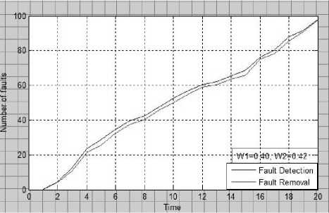
Fig: 1a. Number of fault Vs time.

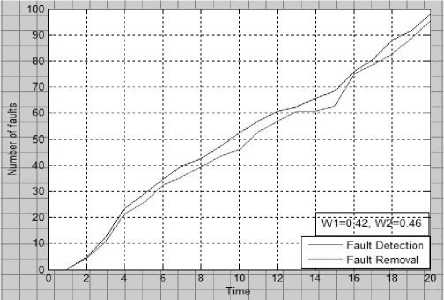
Fig: 1b. Number of fault Vs time.

Above fig. shows the fault detection and correction process Vs time. In first figure we use W1= 0.40 and W2=0.42, in second figure we use W1=0.42 and W2=0.46.

• VII.    Conclusions

In this paper, we propose an alternative foundation for optimal time allocation of fault detection and removal processes using genetic algorithm. We have considered fault detection and removal processes in two stages. During this study we have allocated fault detection and removal processes in dynamic environment. We describe a method to allocate time based on number of faults detected and corrected. This means that the tester and developer can dedicate their time and resources to finish off their testing and debugging tasks for well controlled expenditure. Simulation is done using genetic algorithm, MATLAB and C++ for the same.