Role of information-thermodynamic trade-off models of control qualitative in quantum control algorithm of self-organization design

Author: Barchatova Irina
Journal: Сетевое научное издание «Системный анализ в науке и образовании» @journal-sanse
Article in issue: 3, 2014.
Free access
Different models of self-organization processes are described from physical, information, and algorithmic (quantum computing) point of view. Role of quantum correlation types and information transport in self-organization of structure type design is discussed. A generalized quantum algorithm (QA) design of self-organization processes is developed. Particular case of this approach (based on early developed quantum swarm model) is described. Types of quantum operators as superposition, entanglement and interference in different models evolution of self-organization processes are introduced from quantum computing viewpoint. The physical interpretation of self-organization control process on quantum level is introduced based on the information model of the exchange and extraction of quantum (hidden) value information from/between classical particle’s trajectories in particle swarm. New types of quantum correlations (as behavior control coordinator) and information transport (value information) between particle swarm trajectories are introduced.
Self-organization, quantum control algorithm, stability, robustness, controllability
Short address: https://sciup.org/14123244
IDR: 14123244
Роль информационно-термодинамических моделей распределения качеств управления в проектировании квантового алгоритма управления самоорганизацией
Описываются различные процессы самоорганизации с физической, информационной и алгоритмической (квантового программирования) точек зрения. Рассматривается роль типов квантовой корреляции и информационного обмена в самоорганизации при проектировании структуры квантовой самоорганизации. Приводится общий квантовый алгоритм проектирования самоорганизации, а также частный случай данного подхода. Типы квантовых операторов таких, как суперпозиция, запутанные состояния, интерференция в различных моделях самоорганизации, рассматриваются с точки зрения квантового программирования. Физическая интерпретация процесса самоорганизации на квантовом уровне описывается на основе информационной модели извлечения и обмена квантовой скрытой информации в классических состояниях. Даны новые типы квантовой корреляции и информационного обмена.
Text of the scientific article Role of information-thermodynamic trade-off models of control qualitative in quantum control algorithm of self-organization design
Introduction: Self-organization phenomena
In recent years, the concept of self-organization has been used to understand collective behavior of human being society, animals, ant’s, bird’s, bacteria’s colonies, quantum dots etc. The central tenet of selforganization is that simple repeated interactions between individuals can produce complex adaptive patterns at the level of the group. Inspiration comes from patterns seen in physical systems, such as spiraling chemical waves, which arise without complexity at the level of the individual units of which the system is composed.
Figure 1 is demonstrated the self-organization in different systems. In all these examples, the individual is submerged as the group takes on a life of its own. The individual units do not have a complete picture of their position in the overall structure and the structure they create has a form that extends well beyond that of the individual units. The suggestion is that biological structures such as termite mounds, ant trail networks and even human crowds can be explained in terms of repeated interactions between the animals and their environment, without invoking individual complexity. As examples, a flock of birds twisting in the evening light; a fish school wincing at the thought of a predator; the cram to leave an underground station; ants marching in an endless line; the stop and start traffic jams; the quiet hum of a honey bee hive; the pulsating roar of a football crowd; a swarm of locusts flying across the desert; or even the bureaucracy of the European Union, USA, Japan, China, and Russia.
Q : Beyond the fact that individuals produce collective patterns, is there anything more specific we can say about these phenomena we have labeled self-organized ?
A general characteristic of self-organizing systems is as following: they are robust or resilient . This means that they are relatively insensitive to perturbations or errors, and have a strong capacity to restore themselves, unlike most human designed systems. One reason for this fault-tolerance is the redundant , distributed organization: the non-damaged regions can usually make up for the damaged ones. Another reason for this intrinsic robustness is that self-organization thrives on randomness , fluctuations or «noise». A certain amount of random perturbations will facilitate rather than hinder self-organization. A third reason for resilience is the stabilizing effect of feedback loops.
The present section reviews and analyzed its most important engineering concepts and principles of self-organization that can be used in design of robust intelligent control systems [1].
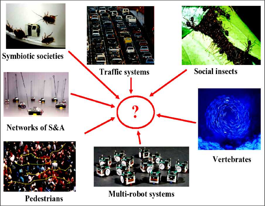
Fig. 3 is demonstrated the main problem of self-organization control.
We choice for analysis of common futures as Benchmarks the following examples [2 – 19]:
-
(1) Pedestrian behavior and self-organization;
-
(2) «Phantom panics» and self-organization;
-
(3) Self-organization of traffic flow models;
-
(4) Swarm self-organization and swarm intelligence (SI):
-
4.1. Applications of SI and ant colony self-organization;
-
4.2. Agent-Based Models (ABM);
-
4.3. Quantum cooperation of two insects;
-
4.4. Engineered self-organization of a bacteria colony;
-
-
(5) Self-organization in nano-scale structures: Quantum corrals .
Briefly physical principles of these self-organization models are described in this paper.
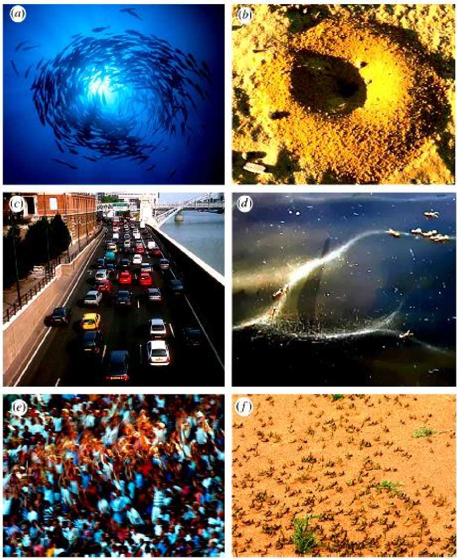
Figure 1. Examples of collective animal behavior:
-
(a) Fish milling (reproduced with permission from Philip Colla, oceanlight.com). (b) The entrance crater to a nest of the ant Messor barbarus (from Theraulaz et al. 2003). (c) Traffic flow in Paris (reproduced with permission from Anthony Atkielski). (d ) A bifurcation in a Pharaoh’s ant trail (reproduced with permission from Duncan Jackson). (e) A Mexican wave at an American football game (taken from Farkas 2002). (f) A band of marching locusts (reproduced with permission from Iain Couzin)
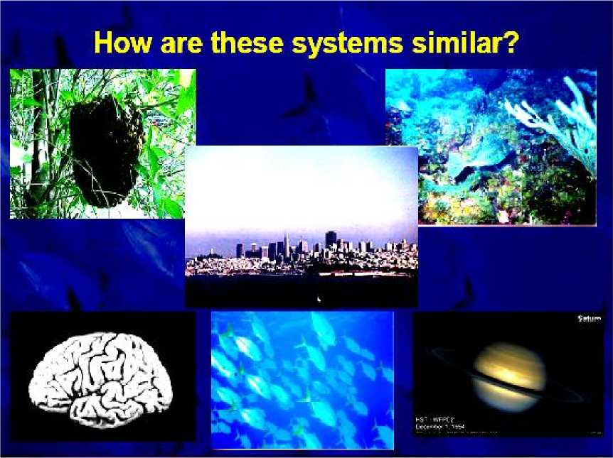
Figure 2. How these systems are similar?
(a)
-
(b)
-
Figure 3. Main problem of self-organization control
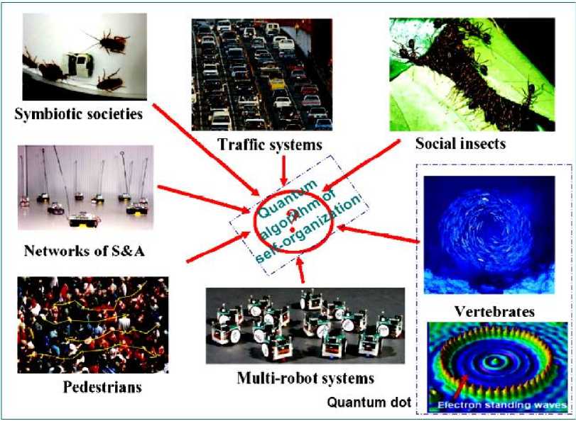
In these examples self-organizational processes begin with the amplification (through positive feedback) of initial random fluctuations. This breaks the symmetry of the initial state, but often in unpredictable (but operationally equivalent) ways. That is, the job gets done, but hostile forces will have difficulty predicting precisely how it gets done. For example, a key issue in nanotechnology is the development of conceptually simple construction techniques for the mass fabrication of nano-scale structures reaching down to the atomic scale. At this level the conventional top-down fabrication paradigm becomes excessively energy-intensive, wasteful, expensive and complicated. The natural alternative is self-organized growth, where nano-scale arrangements are built from their atomic and molecular constituents by processes intrinsically providing structural organization. Fig. 4 is illustrated the self-organization processes on nano-scale levels.
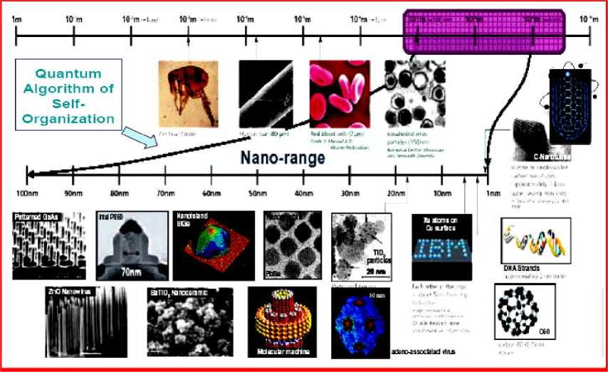
Figure 4. Role of quantum control algorithm in self-organization on nano range
This approach is based on a detailed understanding of the microscopic pathways of diffusion, nucleation and aggregation. The hierarchy in the migration barriers as well as the non-uniform strain fields induced by mismatched lattice parameters can be translated into geometric order and well defined shapes and length scales of the resulting aggregates. In self-organizing systems the relation between cause and effect is much less straightforward: small causes can have large effects, and large causes can have small effects.
This non-linearity can be understood from the relation of feedback that holds between the system’s components. Each component (e.g. a spin) affects the other components, but these components in turn affect the first component. Thus the cause-and-effect relation is circular : any change in the first component is feedback via its effects on the other components to the first component itself.
Remark . The above mentioned feedback is one of important component in advanced control theory and can have two basic values: positive or negative . Feedback is said to be positive if the recurrent influence reinforces or amplifies the initial change. In other words, if a change takes place in a particular direction, the reaction being feedback takes place in that same direction. Feedback is negative if the reaction is opposite to the initial action, that is, if change is suppressed or counteracted, rather than reinforced. Negative feedback stabilizes the system, by bringing deviations back to their original state. Positive feedback, on the other hand, makes deviations grow in a runaway, explosive manner. It leads to accelerated development, resulting in a radically different configuration.
Thus, physically, a process of self-organization typically starts with a positive feedback phase, where an initial fluctuation is amplified, spreading ever more quickly, until it affects the complete system. Once all components have «aligned» themselves with the configuration created by the initial fluctuation, the configuration stops growing: it has «exhausted» the available resources. Now the system has reached equilibrium (or at least a stationary state). Since further growth is no longer possible, the only possible changes are those that reduce the dominant configuration. However, as soon as some components deviate from this configuration, the same forces that reinforced that configuration will suppress the deviation, bringing the system back to its stable configuration. This is the phase of negative feedback.
In more complex self-organizing systems, there will be several interlocking positive and negative feedback loops, so that changes in some directions are amplified while changes in other directions are suppressed. This can lead to very complicated, difficult to predict behavior. These self-organized systems have different physical nature but can be described in general form based on developed quantum control algorithm of self-organization [11].
Analysis of self-organization models gives us the following results.
Models of self-organization are included natural quantum effects and based on the following information-thermodynamic concepts: (i) macro- and micro-level interactions with information exchange (in ABM micro-level is the communication space where the inter-agent messages are exchange and is explained by increased entropy on a micro-level); (ii) communication and information transport on micro-level (“quantum mirage” in quantum corrals); (iii) different types of quantum spin correlation that design different structure in self-organization (quantum dot); (iv) coordination control (swam-bot and snake-bot).
Natural evolution processes are based on the following steps [2–7]: (i) templating; (iii) self-assembling; and (iii) self-organization.
According quantum computing theory in general form every quantum algorithm (QA) includes the following unitary quantum operators: (i) superposition; (ii) entanglement (quantum oracle); (iii) interference. Measurement is the fourth classical operator. [It is irreversible operator and is used for measurement of computation results].
Quantum control algorithm of self-organization that developed below [11] is based on quantum fuzzy inference (QFI) models. QFI includes these concepts of self-organization and has realized by corresponding quantum operators.
QFI is one of possible realization of quantum control algorithm of self-organization that includes all of these features: (i) superposition; (ii) selection of quantum correlation types; (iii) information transport and quantum oracle; and (iv) interference. With superposition is realized templating operation, and based on macro- and micro-level interactions with information exchange of active agents. Selection of quantum correlation type organize self-assembling using power source of communication and information transport on micro-level. In this case the type of correlation defines the level of robustness in designed KB of FC. Quantum oracle calculates intelligent quantum state that includes the most important (value) information transport for coordination control. Interference is used for extraction the results of coordination control and design in online robust KB.
The developed QA of self-organization is applied to design of robust KB of FC in unpredicted control situations. Main operations of developed QA and concrete examples of QFI applications are described.
Principles and Physical Model Examples of Self-Organization
The theory of self-organization, learning and adaptation has grown out of a variety of disciplines, including quantum mechanics, thermodynamics, cybernetics, control theory and computer modeling. The present section reviews its most important definitions, principles, model descriptions and engineering concepts that can be used in design of robust intelligent control systems.
Definitions and main properties of self-organization
Self-organization is defined in general form as following [2, 3, 5, 6]: The spontaneous emergence of large-scale spatial, temporal, or spatiotemporal order in a system of locally interacting, relatively simple components.
Self-organization is a bottom-up process where complex organization emerges at multiple levels from the interaction of lower-level entities. The final product is the result of nonlinear interactions rather than planning and design, and is not known a priori. Contrast this with the standard, top-down engineering design paradigm where planning precedes implementation, and the desired final system is known by design.
Self-organization can be defined as the spontaneous creation of a globally coherent pattern out of local interactions. Because of its distributed character, this organization tends to be robust , resisting perturbations. The dynamics of a self-organizing system is typically nonlinear, because of circular or feedback relations between the components. Positive feedback leads to an explosive growth, which ends when all components have been absorbed into the new configuration, leaving the system in a stable, negative feedback state.
Nonlinear systems have in general several stable states, and this number tends to increase (bifurcate) as an increasing input of energy pushes the system farther from its thermodynamic equilibrium.
Fig. 5 demonstrates this bifurcation situation.
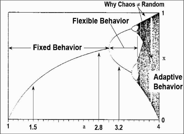
Figure 5. Bifurcation process of non-linear system
To adapt to a changing environment, the system needs a variety of stable states that is large enough to react to all perturbations but not so large as to make its evolution uncontrollably chaotic. The most adequate states are selected according to their fitness, either directly by the environment, or by subsystems that have adapted to the environment at an earlier stage.
Formally, the basic mechanism underlying self-organization is the (often noise-driven) variation which explores different regions in the system’s state space until it enters an attractor . This precludes further variation outside the attractor, and thus restricts the freedom of the system’s components to behave independently. This is equivalent to the increase of coherence, or decrease of statistical entropy , that defines selforganization .
The most obvious change that has taken place in systems is the emergence of global organization. Initially the elements of the system (spins or molecules) were only interacting locally . This locality of interactions follows from the basic continuity of all physical processes: for any influence to pass from one region to another it must first pass through all intermediate regions. In the self-organized state, on the other hand, all segments of the system are strongly correlated . This is most clear in the example of the magnet: in the magnetized state, all spins, however far apart, point in the same direction. Correlation is a useful measure to study the transition from the disordered to the ordered state. Locality implies that neighboring configurations are strongly correlated, but that this correlation diminishes as the distance between configurations increases. The correlation length can be defined as the maximum distance over which there is a significant correlation.
When we consider a highly organized system, we are usually imagined some external or internal agent ( controller ) that is responsible for guiding, directing or controlling that organization. The controller is a physically distinct subsystem that exerts its influence over the rest of the system. In this case, we may say that control is centralized . In self-organizing systems, on the other hand, «control» of the organization is typically distributed over the whole of the system. All parts contribute evenly to the resulting arrangement.
Remark . Although centralized control does have some advantages over distributed control (e.g. it allows more autonomy and stronger specialization for the controller), at some level it must itself be based on distributed control. For example, the behavior of human being body can be best explained by studying what happens in his brain, since the brain, through the nervous system, controls the movement of muscles. However, to explain the functioning of brain, we can no longer rely on some « mind within the mind » that tells the different brain neurons what to do. This is the traditional philosophical problem of the homunculus , the hypothetical « little man» that had to be postulated as the one that makes all the decisions within mental system. Any explanation for organization that relies on some separate control, plan or blueprint must also explain where that control comes from otherwise it is not really an explanation. The only way to avoid falling into the trap of an infinite regress (the mind within the mind within the mind within...) is to uncover a mechanism of self-organization at some level. The brain illustrates this principle nicely. Its organization is distributed over a network of interacting neurons. Although different brain regions are specialized for different tasks, no neuron or group of neurons has overall control.
This is shown by the fact that minor brain lesions because of accidents, surgery or tumors normally do not disturb overall functioning, whatever the region that is destroyed.
As mentioned in Introduction a general characteristic of self-organizing systems is as following: they are robust or resilient . This means that they are relatively insensitive to perturbations or errors, and have a strong capacity to restore themselves, unlike most human designed systems. One reason for this faulttolerance is the redundant , distributed organization: the non-damaged regions can usually make up for the damaged ones. Another reason for this intrinsic robustness is that self-organization thrives on randomness , fluctuations or «noise». A certain amount of random perturbations will facilitate rather than hinder selforganization. A third reason for resilience is the stabilizing effect of feedback loops. Many self-organizational processes begin with the amplification (through positive feedback) of initial random fluctuations. This breaks the symmetry of the initial state, but often in unpredictable but operationally equivalent ways. That is, the job gets done, but hostile forces will have difficulty predicting precisely how it gets done.
Stigmergy is an important principle of self-organization, seen for example in wasp nest building and spider web construction. It refers to a way of coordinating a collective construction process so that the project itself contains the information necessary to guide the actions of the workers. Scientific research has shown the pervasiveness of self-organization in the natural world, from nonliving systems, through microorganisms, to species of all degrees of complexity, including human beings. This research has demonstrated how comparatively simple interactions, often among organisms with limited cognitive capacities, can solve
Электронный журнал «Системный анализ в науке и образовании» Выпуск №3, 2014 год complex command, control, and coordination problems in order to promote their survival and to accomplish their ends.
The behavior of these species is more robust, flexible, and adaptive than they would be if they were not based on self-organization. Self-organization is especially attractive as an approach to the robust, flexible, and adaptive implementation of command, control, and communication systems of enormous potential value to military operations, homeland security, and public safety. With this increased knowledge of natural selforganization, has come improved understanding of various general principles that can be applied to artificial intelligent systems to achieve the same benefits. In past research, a variety of simulation studies have shown that these principles of self-organization can be applied in artificial systems, which may be quite different from the natural systems in which the principles were originally observed.
Principles and Models of Self-Organization
Self-organization has long been a matter of immense interest and research in sociology, anthropology, physics and many other fields. Though the principles of self-organization can be inducted from almost all walks of human, plant and animal lives [2 – 7], and in computer science [8] can be used. It is most evident in ant and termites colonies [9] or self-engineering capabilities of bacteria [10]. Self-organization has been used to explain the formation of cities, software, brain cells and many natural phenomena in human societies. Though the principle is used to explain other phenomena, the concept itself is continuously evolving. Selforganization phenomena are correlated with information transport and thermodynamics processes [5 – 7, 15 – 17].
The term self-organizing systems refers to a class of systems that are able to change their internal structure and their function in response to external circumstances. By self-organization it is understood that elements of a system are able to manipulate or organize other elements of the same system in a way that stabilizes either structure or function of the whole against external fluctuations. Traditionally three qualitative forms of self-organization are analyzed as following:
-
(i) stigmergy ; (ii) reinforcement mechanisms ; and (iii) cooperation .
The amplification phenomena founded in stigmergic process or in reinforcement process are different forms of positive feedbacks that play a major role in building group activity or social organization. Cooperation is a functional form for self-organization because of its ability to guide local behaviors in order to obtain a relevant collective one.
Self-organization mechanisms guide the behavior of the local entities of a collective.
Consequently these approaches allow a drastic reduction of the solution search space compared to global search algorithms. Working on self-organization implies the creation of disorders inside a collective in order to obtain later a more relevant response of the system faced with unexpected events. From an engineering point of view it could be interesting to propose global systems gauges able to link disorder and relevance behavior at the system macro-level.
Self-organization essentially refers to a spontaneous, dynamically produced (re-)organization. Several definitions corresponding to the different self-organization behaviors: (1) Swarm intelligence (SI); (2) Decrease of entropy; (3) Autopoiesis; (4) Artificial systems; (5) Emergence.
Remark . Many natural systems show self-organization property (e.g. galaxies, planets, chemical compounds, cells, organisms and societies). Traditional scientific fields attempt to explain these features by referencing the micro properties or laws applicable to their component parts, for example gravitation or chemical bonds. Furthermore, self-organization implies organization, which in turn implies some ordered structure and component behavior. In this respect, the process of self-organization changes the respective structure and behavior, and a new distinct organization is self-produced. Emergence is the fact that a structure, not explicitly represented at a lower level, appears at a higher level. In the case of dynamic self-organizing systems, with decentralized control and local interactions, intimately linked with self-organization is the notion of emergent properties. The ants actually establish the shortest path between the nest and the source of food. However in the general case, self-organization can be witnessed without emergence and vice-versa.
-
A . Principles of self-organization . Over the last half a century, much research in different areas has employed self-organizing systems to solve complex control problems. However, there is as yet no general
framework for constructing self-organizing systems. Different vocabularies are used in different areas, and with different goals. (Detail description of self-organization principles and different natural/man-manned models of self-organization structures are presented in [3, 5 – 7, 11]). The essence of self-organization is that system structure often appears without explicit pressure or involvement from outside the system. In other words, the constraints on form (i.e. organization) of interest to us are internal to the system, resulting from the interactions among the components and usually independent of the physical nature of those components. The organization can evolve in either time or space, maintain a stable form or show transient phenomena. General resource flows within self-organized systems are expected (dissipation), although not critical to the concept itself.
Remark : Related works . The term self-organization has been used in different areas with different meanings, as is cybernetics, social-economic systems, thermodynamics, biology, mathematics, computing, information theory, synergetic, and others (for a general overview, see [11], and References there). However, the use of the term is subtle, since any dynamical system can be said to be self-organizing or not, depending partly on the observer: If we decide to call a «preferred» state or set of states (i.e. attractor) of a system «or-ganized», then the dynamics will lead to a self-organization of the system. A practical notion will suffice: A system described as self-organizing is one in which elements interact in order to achieve dynamically a global function or behavior [20]. This function or behavior is not imposed by one single or a few elements, nor determined hierarchically. It is achieved autonomously as the elements interact with one another. These interactions produce feedbacks that regulate the system. Many non-living physical and chemical systems have the capacity to generate order from chaos. This capacity is known as self-organization . Self-organized systems can evolve by small parameter shifts that produce large changes in outcome. A common misconception about self-organization in biological systems is that it represents an alternative to natural selection.
Self-organization usually relies on four basic ingredients: (i) Positive feedback; (ii) Negative feedback; (iii) Balance of exploitation and exploration; and (iv) Multiple interactions. All the previously mentioned examples of complex systems fulfill the definition of self-organization.
Fig. 6 shows these principles of self-organization in ant colony. When two food sources of equal quality are offered to an ant society, only one becomes selected through the concurrent influence of positive (in green) and negative (in red) feedback loops. Examples of such feedbacks are given in the Fig. 1. Depending on these feedbacks, the trail amount and hence the probability for newly coming ants to choose one path (either P 1 or P 2) at the bifurcation point will change over time and will ultimately lead to the collective choice of one food source. More precisely, the question can be formulated as follows.
Q : When is it useful to describe a system as self-organizing ?
This will be when the system or environment is very dynamic and/or unpredictable.
If we want the system to solve a problem, it is useful to describe a complex system as self-organizing when the «solution» is not known beforehand and/or is changing constantly. Then, the solution is dynamically strived for by the elements of the system. In this way, systems can adapt quickly to unforeseen changes as elements interact locally. In theory, a centralized approach could also solve the problem, but in practice such an approach would require too much time to compute the solution and would not be able to keep the pace with the changes in the system and its environment. In engineering, a self-organizing system would be one in which elements are designed in order to solve dynamically a problem or perform a function at the system level.
Thus, the elements need to divide, but also integrate, the problem. For example, a swarm of robots will be conveniently described as self-organizing, since each element of the swarm can change its behavior depending on the current situation. It should be noted that all engineered self-organizing systems are to a certain degree autonomous, since part of their actual behavior will not be determined by a designer. In order to understand self-organizing systems, two or more levels of abstraction should be considered: elements (lower level) organize in a system (higher level), which can in turn organize with other systems to form a larger system (even higher level).
The understanding of the system’s behavior will come from the relations observed between the descriptions at different levels. Note that the levels, and therefore also the terminology, can change according to the interests of the observer. For example, in some circumstances, it might be useful to refer to cells as elements (e.g. bacterial colonies); in others, as systems (e.g. genetic regulation); and in others still, as systems coordinating with other systems (e.g. morphogenesis).
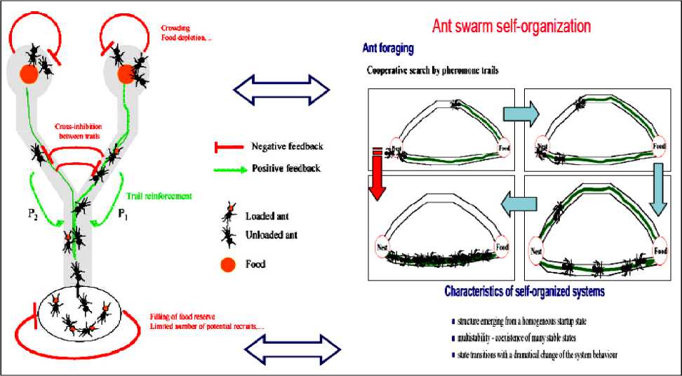
Figure 6. Feedbacks loops and collective choice of one food source (bifurcation) [9]
A system can cope with an unpredictable environment autonomously using different but closely related approaches:
-
- Adaptation (learning, evolution). The system changes its behavior to cope with the change.
-
- Anticipation (cognition). The system predicts a change to cope with, and adjusts its behavior accordingly. This is a special case of adaptation, where the system does not require experiencing a situation before responding to it.
-
- Robustness. A system is robust if it continues to function in the face of perturbations. This can be achieved with modularity, degeneracy, distributed robustness, or redundancy.
Successful self-organizing systems will use combinations of these approaches to maintain their integrity in a changing and unexpected environment. Adaptation will enable the system to modify itself to “fit” better within the environment. Robustness will allow the system to withstand changes without losing its function or purpose, and thus allowing it to adapt. Anticipation will prepare the system for changes before these occur, adapting the system without it being perturbed.
-
B . Elements of self-organization . We can see that all of them should be taken into account while engineering self-organizing intelligent systems.
-
1. Interacting components . The components provide the substrate for organization of higher-level structures. Interaction / communication is necessary for creating linkages to assemble larger structures. Example components are molecules, cells, agents, etc. Example interactions are excitation, inhibition, sensing, attraction, repulsion, etc.
-
2. Constructive processes . Needed to build larger structures from the components, e.g., reproduction, aggregation, crystallization, copying, growth, recombination, ramification, etc.
-
3. Destructive processes . Needed to tear down existing (possibly suboptimal or unwanted) structures to make room for new ones, e.g., death, fragmentation, dissolution, division, mixing, turbulence, noise, etc.
-
4. Autocatalysis/positive feedback . Needed to reinforce and drive the construction of useful structures, e.g., splits encouraging more splitting to create a complex branching structure.
-
5. Homeostasis/negative feedback . Needed to prevent runaway structure formation (e.g., structures beyond a certain size becoming non-receptive to further addition or even unstable).
-
6. Nonlinearity . Needed to magnify some effects and squelch others in order to produce complex structure.
Examples include thresholds, unimodal and multimodal dependencies, saturation, and amplification underlying the constructive, destructive and feedback processes.
What is Emergence?
The appearance of large-scale collective order that cannot be described completely in terms of the individual system components, e.g., meaning from a collection of words, a society from a collection of individuals, a wave from a collection of particles, a picture from a collection of pixels. Emergence seeks to move beyond pure reductionism without resorting to metaphysical explanations, e.g., in explaining phenomena such as intelligence and life. Complex adaptive systems exhibit spontaneous emergence at many levels of description.
-
C. Elements of engineering self-organization design and its role in design of robust intelligent control. Let us consider main approach in engineering philosophy of control design.
Traditional top-down approach:
-
(1) Consider all possibilities; (2) Develop a very careful design; (3) Thoroughly test the design to verify performance; (4) Implement and test a prototype; (5) Carefully replicate the verified design to ensure reliability. This approach relies on anticipation of all eventualities, meticulous design, thorough testing, and exact replication to obtain the desired level of performance. It works best in well-understood, predictable and relatively simple environments.
Self-organized bottom-up approach:
-
(1) Provide the basic elements/components needed; (2) Let the components interact among themselves and with the environment to organize through an iterative process of creative exploration and selective destruction. This approach produces good designs by multi-scale , parallel , intelligent random search through the space of possibilities. It is appropriate (necessary) for large-scale complex systems operating in complex, dynamic, unpredictable environments, e.g., the real world.
Key Difference
Top-Down: Every aspect of the system at all levels is carefully designed and evaluated
-
(a) Non-scalable in cost, time, effort, reliability; (b) Critically dependent on component reliability; (c) Inflexible in response to novel conditions.
Bottom-Up: Only the basic «simple and cheap» components are designed; the rest of the system organizes itself: (a) Inherently scalable; (b) Flexible, robust, versatile, expandable, evolvable.
What do complex adaptive systems buy us?
-
1 . Scalability : The system can grow much larger because no one needs to keep track of everything;
-
2 . Flexibility : The system can change as needed simply by individual agents changing their behavior;
-
3 . Versatility : The system can be used in many different situations without redesign;
-
4 . Expandability : More agents can be added to the system without redesign;
-
5 . Robustness : The system can withstand changes and even loss of individual agents
This is a new kind of engineering:
-
(1) We’re no longer designing the system;
-
(2) We’re engineering the possibility for the system to arise;
-
(3) This will work for some applications and not for others.
Why do we need to build complex adaptive systems?
- To obtain systems with attributes such as intelligence, adaptively, robustness, scalability, and flexibility for operation in complex, dynamic and uncertain environments e.g., battlefields, disaster areas, hazardous regions, ocean floors, outer space, etc.
- To create very large-scale or fine-grained systems where standard design, control, and analysis methods break down for capacity reasons, e.g., sensor networks with millions of nodes, swarms of microsatellites, etc.
- To control other complex adaptive systems, e.g., traffic networks, communication networks, biological systems, etc.
Self-organization may seem to contradict the second law of thermodynamics that captures the tendency of systems to disorder. The «paradox» has been explained in terms of multiple coupled levels of dynamic activity [the Kugler-Turvey model ( Kugler & Turvey , 1987)] self-organization and the loss of entropy occurs at the macro-level, while the system dynamics on the micro-level generates increasing disorder [11, 12, 13, 16, 17].
We are considered five examples of self-organization processes in dynamic systems with different scale dimensions. These examples help to understand main ideas of self-organization and find mutual components of quantum control algorithm of self-organization design.
In next sections the structure of this quantum design algorithm and its application to design of robust knowledge base in intelligent FCs are considered.
Simulation results are considered on examples of essentially non-linear dynamic system control objects.
Model’s analysis of self-organization processes
Analysis of self-organization models in this section gives us the following results.
-
1 . Natural evolution processes are based on the following steps [2–7]:
-
(i) templating ; (iii) self-assembling ; and (iii) self-organization .
-
2 . Models of self-organization are included natural quantum effects and based on the following information-thermodynamic concepts:
-
(i) macro- and micro-level interactions with information exchange (in ABM micro-level is the communication space where the inter-agent messages are exchanged and is explained by decreased entropy on a macro-level and increased entropy on a micro-level);
-
(ii) communication and information transport on macro- and micro-levels (“quantum mirage” in quantum corrals);
-
(iii) different types of quantum spin correlation that design different structure in self-organization (as example, quantum dot);
-
(iv) coordination control (swam-bot and snake-bot).
-
3 . Quantum control algorithm of self-organization that developed below [11] is based on quantum fuzzy inference (QFI) models. QFI includes these concepts of self-organization and has realized by corresponding quantum operators.
Let us consider the common parts of models of self-organization processes of natural evolution processes according to abovementioned Items 1 and 2 of our results.
Main common parts in evolution self-organization processes of Nature. Main steps of generalized (bioinspired) self-organization processes are as following:
-
- First step is a templating that is organization of component by a template ;
-
- The second step is a self-assembly with control via conformation;
-
- The third step is a self-organization as collective behavior of interactive (possible self- assembly) components.
From the description of qualitative properties of these models we can extract common parts. Main common parts of self-organization processes (described in details in [11]) are as following: (1) Presence of different type correlations (spatial, temporal, or spatiotemporal types); (2) Random search in design process of a new structure in accordance with initial state and fixed correlation type; (3) Robustness of final new structure; (4) Flexibility of self-organized structure.
These common parts are used in bio-inspired and man-made self-organization process (see, Fig. 7).
Fig. 7 shows also the structure and the main steps (right column) of bio-inspired self-organization processes in things natural and things man-made.
Let us consider one of simple examples of natural self-organization with natural operators.
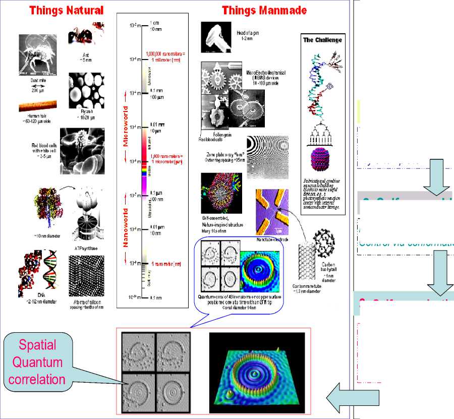
Figure 7. Structure of self-organization processes in things natural and things manmade and selforganization evolution
Steps of Bio-Inspired Self-Organizatio Evolution
1. Templating
Organization of molecular component by a template
2. Self-assembly
---------------------------------1
Molecular self-assembly; i
Control via conformation I
3. Self-organization
---------------------------------1
Collective behavior of i interactive I
(possible self-assembly) !
components 1
Example : Crowd behaves as excitable media during Mexican wave . Mexican wave, or La Ola, first widely broadcasted during the 1986 World Cup held in Mexico, is a human wave moving along the stands of stadiums as one section of spectators stands up, arms lifting, then sits down as the next section does the same (see, Figs 8 and 9a).
Remark. Here we are used variants of models originally developed by I. Farkas, D. Helbing and T. Vicsek (1994) for the description of excitable media to demonstrate that this collective human behavior can be quantitatively interpreted by methods of statistical physics. Adequate modelling of reactions to triggering attempts provides a deeper insight into the mechanisms by which a crowd can be stimulated to execute a particular pattern of behavior and represents a possible tool of control during events involving excited groups of people. Using video recordings it was analyzed 14 waves in stadiums with above 50.000 people: the wave has a typical velocity in the range of 12m/s (20 seats/s), a width of about 6-12m (~15 seats) and more frequently rolls in the clockwise direction. It is generated by the simultaneous standing up of not more than a few dozens of people and subsequently expands over the entire tribune acquiring its stable, close to linear shape (see dedicated to the present work, offering further data and interactive simulations).
The relative simplicity of the Mexican wave allows us to develop a quantitative treatment of this kind of collective behavior by building and simulating models accurately reproducing and predicting the details of the associated human wave. We show here that the well-established approaches to the theoretical interpretation of excitable media – originally created for describing such processes as forest fires or wave propagation in heart tissue – can readily be generalized to include human social behavior.
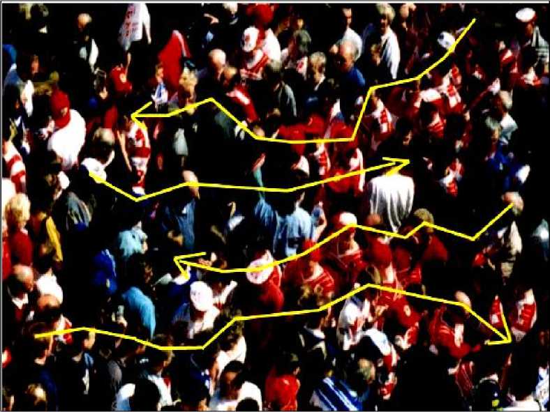
Figure 8. A human wave moving along the stands of stadiums
It was developed two mathematical simulation models, a minimal and a more detailed one to demonstrate the robustness of self-organization approach.
Model : If the weighted concentration of active people within a radius of R around a person is above the threshold of the person ci (randomly chosen from [ c-Dc, c+Dc ]) then the person is activated. Weights decrease exponentially with distance and changed linearly with the cosine of the direction so that people on the left of a person have an influence w0 times as strong as those on the right. The direction of the wave’s motion is determined by this anisotropy due to spontaneous symmetry breaking at the early stages resulting from anticipation and the anisotropy in perception since the majority of people are right handed. Group trying to induce a wave and the average threshold c. Parameters are as above, and each point represents the average of 128 simulations.
In analogy with models of excitable media, in both versions people are regarded as excitable units: they can be activated by an external stimulus (a distance and direction-wise weighted concentration of nearby active people exceeding a threshold value c ). Once activated, each unit follows the same set of internal rules to pass through the active (standing and waving) and refractory (passive) phases before returning to its original, resting (excitable) state. While the simpler version distinguishes three states only (excitable/active/passive) and accounts for variations in the individual behavior by means of transition probabilities between the states, the elaborate version takes into account an actual, deterministic activity pattern in more detail.
The two versions of the model we considered differ in the way stochasticity, i.e., differences and fluctuations regarding the above behavioral patterns are represented (for details see .
Next, we employed these models to get an insight into the conditions for triggering a wave. Figure 9b shows the evolution of a wave provoked by the simultaneous excitation (standing up) of a small group of units (people). Using parameters deduced from video recordings for the sizes and characteristic times of the phenomenon (interaction radius, reaction/activation times and probabilities) we have been able to reproduce the above described observations concerning the size/form/velocity and stability of the wave.
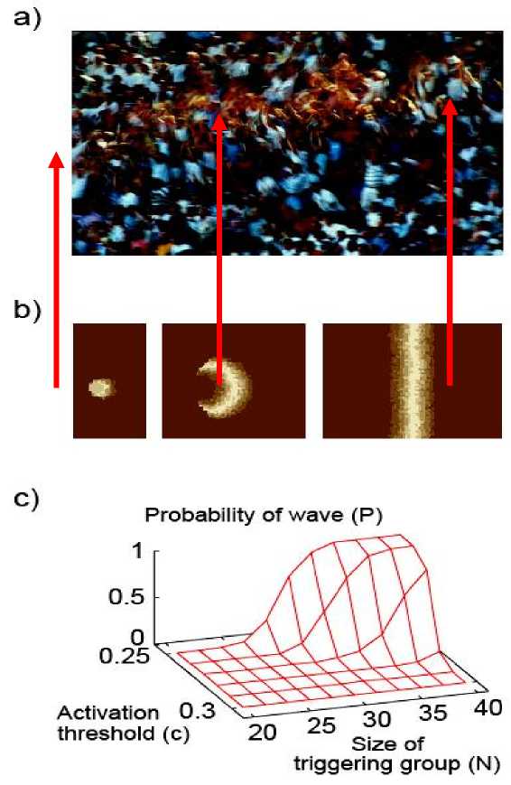
Figure 9. Photo and simulations of the Mexican wave
-
(a) Photo of a Mexican wave; (b) Snapshots of the n state model, where, after activation, a person deterministically goes through na active states (stages of standing up) and nr refractory states. The wave is shown at 0.5s, 2s, and 15s after the triggering event on a tribune with 80 rows of seats. Brighter shades correspond to higher level of activity. Parameters are na = nr = 5, c = 0.25, Dc = 0.05, R = 3 and w0 = 0.5; (c) P(N, c), the ratio of successful triggering events, as a function of the number of people N in the group trying to induce a wave and the average threshold c.
Fig. 9c displays the probability of generating a wave when a small group of varying size tries to trigger it under different excitation threshold values.
The results clearly demonstrate that the self-organization dependence of the eventual occurrence of a wave on the number of initiators is a rather sharply changing function, i.e., triggering a Mexican wave requires a critical mass. The present approach is expected to have implications for the treatment of situations where influencing the behavior of a crowd is desirable. In particular, in the context of violent street incidents associated with demonstrations or sport events, it is essential to know under what conditions groups can gain control over the crowd and how fast and in which form this perturbation/transition can spread.
Example: The collective behavior of humans within crowds. In our earlier discussion of humans we considered the case where people interact through environmental modification (trail formation), and largely ignored the influence of direct interactions among pedestrians. However, within urban setting individuals can seldom influence their surroundings in this way. Furthermore, when walking down a busy street, or corridor, one balances global goal-oriented behavior (desire to reach a certain point) with local conditions created by the motion and positions of other nearby pedestrians. Each member in such a crowd is likely to have a lim- ited perceptive radius in which information to determine future movement must be gathered. Consequently, larger scale patterns in crowds are seldom evident from an individual pedestrian’s viewpoint.
However, if viewed from above crowds often do display obvious and consistent patterns. One of the most common of these can be seen when there is bi-directional traffic, as for example when people are trying to move both ways along a walkway, or crossing the road at a crosswalk. Under such circumstances ‘bands’ of pedestrians form: each band composed of a number of pedestrians with a common directional preference ( Milgram and Toch , 1969).
Fig. 10a demonstrates this situation.
Remark . The flow of pedestrians under conditions of crowding was likened by Henderson (1971) to the motion of fluids or gases. He used a well-known technique for the mathematical analysis of such materials, the Navier-Stokes equation for fluid dynamics, to simulate a crowd. Although providing an insight into how individual-level (microscopic) properties lead to large-scale (macroscopic) properties, such an approach is difficult to implement since the conservation of energy and momentum assumptions for a physical system do not apply to a biological system in which the individual components are «self-driven». Despite this, Helbing (1992) was able to modify such equations with respect to some of these properties, but analytic solutions proved hard to find. The most promising approach to studying crowd behaviors comes from individual-based modeling.
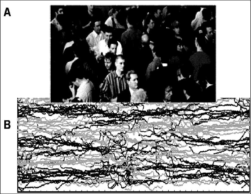
Figure 10. Simulation of pedestrian dynamics showing lane formation (from Couzin, 1999).
The successive positions (trajectories) of individuals with a desire to move to the left are shown in gray.
The positions of those individuals intending to move to the right are shown in black
Influence of repulsion (collision avoidance). Helbing and Molnár (1995) developed a simple individualbased model of pedestrian motion in which they consider people moving in opposite directions along a corridor. This simple geometric representation of space allows the assumption that all individuals have a desire to move only in one direction or another along the walkway. However, pedestrians will also tend to avoid collisions by decelerating and turning away if they come into close contact with one another. When no other individuals are within a specified local range, individuals will tend to accelerate to a desired speed, and orient towards their destination. This simple behavioral response alone can account for the formation of bands when there is bi-directional traffic. Individuals meeting others head on will have «strong» interactions in which they are likely to slow down and move aside to avoid collisions. Initially this occurs frequently. How- ever, individuals that find themselves behind others moving in the same direction are less likely to have to perform such extreme avoidance maneuver, and in turn they «protect» others behind them, from head on avoidance moves. Given a sufficiently long corridor (and a sufficiently high traffic flow for interactions among pedestrians to be an important factor) the system will self-organize into lanes. Individuals entering the corridor (at random positions) move around in the direction perpendicular to their desired direction of travel when they interact with oncoming pedestrians. However, if by chance they fall in behind another individual moving in the same direction this is a more «stable» state.
Thus the system naturally self-organizes into a situation where pedestrians are in the «slipstream» of others moving in the same direction as themselves, thus creating bands, and reducing movement in the direction perpendicular to desired motion (see, Fig. 10b). Helbing and Molnár (1995) also demonstrated in their model that the number of bands that tend to form scales linearly with the width of the walkway.
This demonstrates that there is a characteristic length-scale to the pattern-forming process: that is, from any point in the system statistically similar motions is occurred one wavelength away.
Influence of attraction to other pedestrians . Clearly one does not need to invoke complex individual behavior to explain the banding patterns found in human crowds. The above model shows how individuals would «naturally» occupy space (in the dimension perpendicular to desired direction of travel) in which others ahead and behind them tend to have a similar direction of motion. It is possible in real crowds, however, that individuals actively (as well as passively) seek such positions. That is, instead of finding such positions by chance, as in the previous model, they will tend to deliberately walk behind individuals moving in the same direction as them selves. For example, Couzin (1999) simulated the motion of pedestrians crossing a road at a crosswalk. Given the type of rules described above the system requires some time to «find» the collision-minimization state. Consequently, in the crosswalk situation, although some banding does occur, congestion is still relatively high (Fig. 11a). However, if one adds a supplementary rule such that an individual will exhibit a propensity to follow other individuals moving in their desired direction, then bands tend to form much more readily, thus reducing head-on collisions and increasing the rate of flow (Fig. 11b). On a crosswalk, such bands begin to form even before the pedestrians moving in different directions meet. Thus the groups act as «wedges» when they come into contact with one another allowing the bands to interlace more readily when they reach the central area of the walkway. Thus, although attraction is not a necessary condition for bands to form in crowds, it decreases the time taken for bands to develop, and increases the flow rate more rapidly than does avoidance alone.
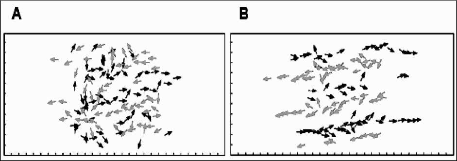
Figure 11. Simulation of pedestrians attempting to move across a crosswalk
-
(a) where individuals just exhibit repulsion from others flow is less smooth than when, (b) they exhibit repulsion but also attraction towards others that have a similar desired direction [Gray – individuals intending to move left. Black – individuals attempting to move right]
The influence of the geometry of the environment. In these pedestrian models, the geometry of the environment is very simple. However, what happens when one introduces an obstacle within the environment? Helbing and Molnár (1995) investigated how their model behaved when they placed a doorway in the corridor. What they found was that, given a sufficient density of pedestrians, oscillations in alternating flows of passing direction at the doorway occur. This occurs because the “pressure” of pedestrians at one side of the door eventually results in an individual being able to make it through the door. This makes it easier for indi- viduals with the same desired direction to follow, resulting in a unidirectional flow of individuals through the doorway, as shown in Fig. 12.
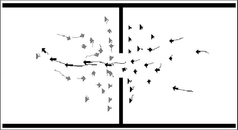
Figure 12. Simulation of pedestrians at a doorway exhibiting oscillations of flow
Remark. In Fig. 12 individuals moving to the left have temporarily monopolized the doorway. The decrease in «pressure» to the right of the door, caused by this exodus, will shortly allow those standing to the left of the doorway to block, and then to temporarily monopolize the doorway, and so on. Image modified from the simulation results that available from at
This reduces the «pressure» of pushing pedestrians at that side of the door, which will then result in a situation where the flow is stopped, and then individuals moving in the other direction are able to pass through (since the «pressure» on their side is now greater), and so on. If the doorway is widened, changes in direction of flow become more rapid. It was also found that, given the same total width of doorway, two half-sized doors near the walls of the corridor increase the rate of flow of pedestrians relative to a single door. This is because, due to the mechanism of band-formation described above, each door becomes used by pedestrians flowing in a common direction for relatively long periods of time. Individuals leaving their respective doorway in one direction «clear» the space ahead of the door for their successors.
Crowd behavior and emergency situations . Under certain extreme conditions, such as when people are evacuating from a crowded building, panic can result in pedestrians being injured or killed through crushing or trampling. In some cases crushing can occur in the absence of any external factor (e.g. fire) resulting instead from the impatience of queuing individuals, who having predominantly only local information, push forward. The physical interactions among members of a crowd can add up to because dangerous pressures up to approximately 4,450 Nm -1 , which can cause brick walls to collapse, bend steel barriers, and result in a large number of fatalities ( Elliott and Smith , 1993). In an attempt to understand better such collective situations, Helbing et al . [4] extended their models of pedestrian behavior to include a «body force», which counteracts the compression of bodies, and a «sliding friction force» which impedes relative tangential motion within crowds. Furthermore, they assume that, within such crowd situations, people exhibit a greater degree of stochasticity (fluctuations) in their movement, and a higher desired velocity, due to the psychological effects of panic ( Kelly et al. , 1965). The model showed that increasing the value of either, or both, of these parameters caused an increase in evacuation time from a building by increasing the degree of interpersonal friction. This resulted in blockages which occurred especially in the vicinity of bottlenecks. Thus, people fleeing from a building can decrease their chances of survival by attempting to move as fast as possible, or by performing uncoordinated movement through nervousness or panic.
Within conditions where individuals have very restricted information about their local surroundings, such as in a smoke-filled room, Helbing et al . [4] investigated the possibility that people may respond not only individualistically, but also in response to the motion of individuals near them, which they term a «herd-ing effect». Under such conditions neither pure individualism nor herding behavior performs well. Following just the individualistic rule, the discovery of an exit becomes a largely random process for each individual.
Although herding can result in groups of individuals escaping if an exit is found, it is more likely that the crowd will move in the same, blocked, direction.
However, if people are assumed to use an intermediate strategy combining both individualism and herding, then the rate of escape is maximized, given the assumptions of the model. These models of human crowds are based on a simplified set of plausible interactions, and as such provide useful insights into the general behavior of such groups under a variety of conditions. There is, however, a need for further empirical studies, which are lacking despite the economic and/or social benefits of such research (e.g. in designing facilities so to reduce risk during evacuation). We encourage initial studies to be made of crowds within relatively simple environments, such as on walkways, where an individual’s desired direction of travel can be better judged than for example in a crowded street, where motivations may change dynamically and be influenced by many more factors.
Modelling a crowd composed of discrete individuals rather than a continuous fluid clearly brings added complications. Helbing et al . model «non-fluid» crowd properties, such as the «faster-is-slower» phenomenon in which people in a rush end up going slower. They also investigate the best evacuation strategy for people in a smoke-filled room (see, Fig. 13).
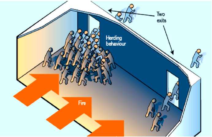
Figure 13. How crowd behavior affects escape from a smoke-filled room
Previous simulations of pedestrian behavior in crowds have used a model based on fluid flow through pipes, but these ignored the actions of individuals. According to the individual-centered model of Helbing et al. [4], the evacuation of pedestrians from a smoke-filled room with two exits can lead to herding behavior and clogging at one of the exits. By contrast, a traditional fluid-flow model would predict the efficient use of both exits. A more individual-centered approach is required to reproduce the behavior of real crowds. Such information can then be used to work out low-risk designs for the width of corridors, the number and position of doors, and the size of areas where people may gather. But these types of study can also provide us with a wider range of possible solutions to crowd problems. The crowd composed of individual people can respond to information directed towards them, to help them choose the most appropriate direction to take or the most appropriate exit to use.
Gathering data during genuine evacuation procedures will always be problematic (practically, and in some cases ethically), but data gathered from practice evacuations may be very useful in testing, and further improving, current models. The importance of such safety issues has been further emphasized by the events of September 11 th 2001 where large, highly populated buildings («The World Trade Center» in New York and «The Pentagon» in Washington D.C.), and the streets around these buildings, had to be evacuated.
Remark. The model presented by Helbing et al. is just one of many possible models. To decide whether a particular model is an accurate description of real life, or to determine which model is the «best» for the situation under consideration, requires real data to compare with each model’s predictions. But such data are scarce or non-existent and may be extremely difficult to collect. With any type of mathematical modeling we always have to be careful to distinguish between «real life» and our attempt to model it. Failing to recognize this difference can have serious consequences. But provided we are aware of when it is appropriate to use a particular model, it can provide valuable information to guide the planning process, for construction and for dealing with emergencies. Perhaps perfect safety is unattainable, but improved models of crowd dynamics can help to increase our safety in crowded situations.
Example . One of the most unexpected phenomena predicted by Helbing et al. is the symmetry breaking in the escape from a room with two identical exits. Here we describe experiments on ants that corroborate this behavior and show that the escape dynamics of ants under controlled panic can serve as a model to study humans in analogous situations. In a first type of experiments (Experiment I), it was introduced a group of approximately 80 individuals of the ant species Atta insularis collected from natural nests, into a circular cell covered by a glass plate with two exits symmetrically situated at left and right (see, Fig. 14a), which were initially blocked.
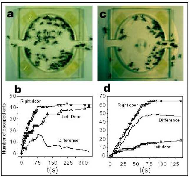
Figure 14. Escape of ants from a cell with two symmetrically located exits
Experiment detail description (E. Altshuler, O. Ramos, Y. Nuñez & J. Fernández, Panic-induced symmetry breaking in escaping ants , 2005). The cell consists in an acrylic drum of 80 mm diameter and 5 mm height, with two exits 10 mm wide symmetrically situated at left and right positions. The drum rests on an circular piece of filtering paper laying on an horizontal surface, and is covered by a flat glass plate of 3 mm thickness with a hole of 2 mm diameter situated at the center of the drum. Approximately 80 ants from the species Atta insularis are added with both exits blocked by acrylic bars. (a); ant distribution several seconds after opening the exits at t = 0. (b); number of ants abandoning the cell as time goes by. (c); ant distribution several seconds after adding 50 ml of an insect repellent fluid ( Citronela , Labiofam, Cuba) though the central hole, and then opening the exits at t = 0 (note a circular spot of repellent fluid of approximately 20 mm diameter at the centre of the cell) (d). Clogging of ants at the right exit is clearly visible (d), number of ants abandoning the cell as time goes by, quantitatively demonstrating the symmetry breaking when repellent is added. Small deviations from the ideal circular shape of the repellent spot or from its location at the center of the setup did not produce important effects in the experimental output. Then, we opened the exits synchronously, and counted the number of ants abandoning the cell through each exit until it was empty.
Fig. 14b shows a graph describing quantitatively the result of a sample run of Experiment I. Although the difference in the use of the two doors eventually reaches a value of 15 ants at a certain stage of the run (roughly corresponding to 20% of the total of escaping ants), it becomes clear that both doors have been used almost symmetrically at the end.
A very different output, however, results from a second kind of experiments (Experiment II). In this case everything takes place as in Experiment I, with the important difference that, a few seconds before opening the doors, a dose of 25 or 50 ml of an insect repelling liquid is rapidly injected in the cell through a hole in the covering glass, producing a disk-shaped spot of the substance at the center of the filtering paper on which the whole setup rests (Fig. 14c). A sample output of Experiment II is shown in Fig. 14d. Differently from Experiment I, one of the doors is always much more used to escape than the other one, which can be described as a symmetry breaking induced by «panic» associated to the repelling agent. In the specific run depicted in Figs 14c,d the difference in the use of the two doors reached nearly 50 ants at the end of the experiment (around 60% of the total number of escaping ants). Besides symmetry breaking, a second difference between Experiment I and II clearly seen in Fig. 14b, d is that, in the latter, the total time of escape is much smaller, probably because the «desired velocity» of the ants increases due to the effect of the repelling agent. Similar results were observed in several runs of Experiment I and II: statistics showed that the difference in use between the two exits at the end of the experiment were, in average, 12% for Experiment I and 51% for Experiment II. The «preferred exit» in Experiment II was either the left or the right one, with no connection to any source of asymmetry in the experimental set-up or to the spatial distribution of ants inside the cell before opening the doors.
The experimental results were also quite similar when using ants collected from the same nest, or from different nests no more than 20 meters apart from each other. They were also similar when repeated on the same group of ants.
These results are coherent with the theoretical predictions reported by Helbing et al. They defined a «panic parameter» which induces individualistic behavior (each pedestrian tends to find an exit by him/herself) when low, and herding behavior (pedestrians tend to follow the crowd) when high. In their two-exit room simulations, the authors find that a high value of the panic parameter produces jamming at one of the doors, thus provoking inefficient escape.
This tendency shows that their panic parameter is related to the effect of the repelling substance used in experiments. In spite of the huge behavioral differences between humans and ants in normal conditions10, experiments suggest that some features of the collective behavior of both species can be strikingly similar when escaping under panic.
Applications of swarm intelligence (SI) and ant colony self-organization . Wasps, bees, ants and termites all make effective use of their environment and resources by displaying collective SI. Termite colonies – for instance – build nests with a complexity far beyond the comprehension of the individual termite, while ant colonies dynamically allocate labor to various vital tasks such as foraging or defense without any central decision-making ability. Recent research suggests that microbial life can be even richer: highly social, intricately networked, and teeming with interactions, as found in bacteria. What strikes from these observations is that both ant colonies and bacteria have similar natural mechanisms based on Stigmergy and SelfOrganization in order to emerge coherent and sophisticated patterns of global foraging behavior. Keeping in mind the above characteristics a Self-Regulated Swarm (SRS) algorithm was proposed which hybridizes the advantageous characteristics of SI as the emergence of a societal environmental memory or cognitive map via collective pheromone laying in the landscape (properly balancing the exploration/exploitation nature of our dynamic search strategy), with a simple Evolutionary mechanism that trough a direct reproduction procedure linked to local environmental features is able to self regulate the above exploratory swarm population, speeding it up globally. In order to test his adaptive response and robustness, it has recurred to different dynamic multimodal complex functions as well as to Dynamic Optimization Control problems, measuring reaction speeds and performance. Final comparisons were made with standard Genetic Algorithms , Bacterial Foraging strategies , as well as with recent Co-Evolutionary approaches. SRS ’s were able to demonstrate quick adaptive responses, while outperforming the results obtained by the other approaches. Additionally, some successful behaviors were found: SRS was able to maintain a number of different solutions, while adapting to unforeseen situations even when over the same cooperative foraging period, the community is requested to deal with two different and contradictory purposes; the possibility to spontaneously create and maintain different subpopulations on different peaks, emerging different exploratory corridors with intelligent path planning capabilities; the ability to request for new agents (division of labor) over dramatic changing periods, and economizing those foraging resources over periods of intermediate stabilization. Finally, results illustrate that the present SRS collective swarm of bio-inspired ant-like agents is able to track about 65% of moving peaks traveling up to ten times faster than the velocity of a single individual composing that precise swarm tracking system. This emerged behavior is probably one of the most interesting ones achieved.
Example . Networks that control the flow of resources and information are ubiquitous in nature. Moreover, the efficiency of such networks may determine the fundamental scaling properties of certain organisms. The foraging networks of terrestrial animal societies, and especially those of certain ant species, provide unrivalled opportunities to quantify both the behavior of individual items of traffic and the larger-scale patterns of traffic flow. For these reasons, they are ideal subjects with which to test mathematical models that link the behavior of small components (in this instance, individual ants) to the overall efficiency of the dynamic structures they generate.
Many ant species create chemical (pheromone) trail networks, not only to transport resources and/or information swiftly and efficiently during foraging, but also for exploration, emigration and coordinating colony defense ( Holldobler & Wilson , 1990). Just as the functioning and success of modern cities are dependent on an efficient transportation system, the effective management of traffic is also essential to insect societies. The flow of traffic along trails is likely to be particularly important in the New World army ant Eciton burchelli . Colonies of this species may have half a million or more workers, and the ants are strict carnivores. They stage huge swarm raids, in pursuit of arthropod prey, with up to 200 000 virtually blind foragers forming trail systems that are up to 20 m wide and 100 m or more long ( Schneirla , 1971; Franks et al. 1991; Gotwald 1995; Sole ´ et al . 2000). In a single such raid a colony may retrieve more than 30 000 prey items ( Franks 1985). Moreover, these massive raids are severely time constrained. At most, they begin at dawn and end at dusk, when the colony emigrates, under the cover of darkness, to a new nest-site and foraging arena.
For this reason, E. burchelli colonies need to operate at a very high tempo (see Franks et al. 1999; Boswell et al. 2001). These colonies form traffic lanes in their main foraging columns ( Franks 1985). It was investigated how and why these traffic lanes form. It was shown how the movement rules of individual ants on trails can lead to a collective choice of direction and the formation of distinct traffic lanes that minimize congestion. The results of a new model with a quantitative study of the behavior of the army ant Eciton burchelli was developed and evaluated. Colonies of this species have up to 200 000 foragers and transport more than 3000 prey items per hour over raiding columns that exceed 100 m. It is an ideal species in which to test the predictions of the model because it forms pheromone trails that are densely populated with very swift ants. The model explores the influences of turning rates and local perception on traffic flow. The behavior of real army ants is such that they occupy the specific region of parameter space in which lanes form and traffic flow is maximized.
Remark . Lane formation is also known to emerge spontaneously in human crowds under certain conditions. Where there is bi-directional traffic (such as on a walkway or crosswalk) «bands» of pedestrians can form, each band composed of pedestrians with a common directional preference ( Milgram & Toch 1969). These large-scale patterns are seldom evident to an individual pedestrian because they often have a limited perceptive radius in which information to determine future movement must be gathered. Like army ants, pedestrians in crowds balance goal oriented behavior (desire to reach a destination) with local conditions created by the motion and positions of nearby pedestrians (avoidance of collisions). It is the balance of these «so-cial forces» that results in lane formation. Individuals meeting others head-on will have «strong» interactions in which they are likely to slow down and turn away to avoid collisions. Individuals that find themselves behind others moving in the same direction as themselves are less likely to perform such extreme avoidance maneuvers, and, in turn, they «protect» others behind them from head-on avoidance moves, increasing the flow rate. Thus, given a sufficient density of pedestrians, they will spontaneously form lanes ( Helbing & Molna'r 1995). The number of lanes that form in human crowds scales linearly with the width of the walkway ( Helbing & Molna ´r 1995). Thus, there is a characteristic length-scale to this pattern-forming process: that is from any point in the system statistically similar motions occurred one wavelength (lane width) away (in the direction perpendicular to the desired motion). This is in contrast to the fixed three-lane system of army ants, which results from the asymmetry in interactions (absent in human crowds) combined with a tendency for all ants to move towards the highest concentration of pheromone. A further difference between ants and humans is that pedestrians can typically be expected to behave selfishly. That is, they will tend to minimize their own travel time, but this may be at the cost of others. An army ant colony, however, is composed of cooperative individuals. Thus, natural selection can build an adaptive pattern at the global level by selecting and modifying individual rules that encode collective patterns. The asymmetry in interactions we have revealed is therefore likely to have been selected for. However, there is another potential explanation that is not mutually exclusive: many ants returning to the nest are burdened with prey, and this may make them less maneuverable than unladed ants leaving the nest.
Why do army ants have a three-lane structure as opposed to one with just two lanes ?
Let us consider two models of ant’s motion behavior.
-
(i) Collective selection of a direction . The collective properties of the model during the generation of spatial pattern over a short but representative section of trail (equivalent to 50 cm) are investigated. Army ants are not only good at following trails but also have a propensity to form circular mills when moderate numbers are separated from a colony and restricted to a confined area, either in the laboratory (see, Figure 15 a ) or naturally in the field during exceptionally severe rainstorms ( Schneirla 1971; Franks et al. 1991; Gotwald 1995).
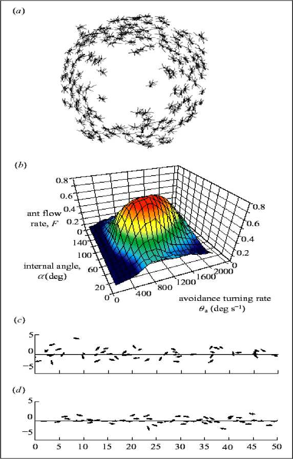
Figure 15. Circular milling
(a) Drawing of ants forming a circular mill in the laboratory (adapted from Schneirla 1971 by I.D.C.);
(b) The flow of ants is dependent on their ability to detect others and the rate at which they turn during avoidance maneuvers (N = 50, Qp = 500° s - 1 , ст = 0.01, Q = 1.2 x 10 - 6 g cm - 3 , C^ = 1.2 x 10 - 6 g cm - 3 , τ = 300 s. F was calculated at t = 5000, and the results shown are the means of 100 runs per parameter combination); (c) Ants begin the simulation at random positions and with orientations along the trail. Snapshot near the start of a simulation (t = 50) with a = 90° and 0a = 1000° s - 1 . Ants are depicted as arrows representing their instantaneous velocity (units: cm); (d) Simulated ants have selected a direction collectively (t = 3000)
After a period of disorder, the ants all begin moving in the same direction. This behavior is likely to reflect the ability of army ant colonies collectively to select a raid direction. Periodic boundary conditions are used, which make the simulation very similar to the circular mill, and investigate how the model parameters influence the collective behavior of ants on the trail section.
The flow of simulated ants, F , (measured as the normalized magnitude of the sum of the velocities of all individuals; values close to 0 represent little flow in a given direction, and those close to 1 represent high flow in one direction) is influenced strongly by the avoidance turning rate, θ , and the internal angle of the perception zone ahead of an ant, α (see, Fig. 15b). High flow rates occur when the ants select a direction collectively (see, Figs 15c, d). When θ a low, ant is require repeated collisions with others before their trajectory is influenced strongly enough for them to turn around. This causes congestion because ants turn slowly when they detect others, and, consequently, must slow down to avoid collisions. Conversely, when θ is very high, ants are change direction very quickly when others are detected, and their orientations do not become correlated. Similarly, when α a low, ant is cannot detect others ahead of them adequately, and are thus relatively insensitive to the positions of others. If α is high, however, they spend much of their time avoiding individuals that they would be unlikely to collide with. At intermediate values of these parameters ants are sufficiently sensitive, yet not overly sensitive, to the positions of others and, consequently, can select a direction collectively (hereafter α = 90°). In this region of parameter space stochastic fluctuations in the number of ants traveling in each direction leads to one direction being more common than the other. This change causes an autocatalytic behavioral response as ants opposing the main flow are forced to turn around through repeated head-on interactions. As more ants move in one direction, it becomes increasingly hard for individuals to move the opposite way, and this causes the ants collectively to select a (randomly determined) direction.
-
(ii) Bi-directional traffic and lane formation . The results of the model suggest that army ants have evolved a behavioral response that results in a general tendency for them to all moves in the same direction along a trail. Under natural conditions, certain army ants exhibit a predominantly unidirectional flow of workers away from the nest in the first stage of a raid, but, as an increasing number of ants return to the nest carrying prey, the flow of ants in the raiding columns becomes bi-directional. In the sections of principal trails of the army ant E. burchelli that was filmed, the ants exhibited a distinct spatial structuring, with ants leaving the nest predominantly using both margins of the trail and ants returning to the nest using the centre.
How do E. burchelli army ants form traffic lanes? Can this difference in turning rate account for the pattern seen? (I. D. Couzin and N. R. Franks, «Self-organized lane formation and optimized traffic flow in army ants», Proc. R. Soc. Lond., B, 2002).
It was assumed that the ants have a sense of direction ( Gotwald , 1995). Hence, each simulated ant is now supplied with a supplementary internal directional vector that is parallel to the trail, pointing either to the left (returning towards a «nest») or to the right (outbound towards a «foraging area»). N /2 ants have a preference to move in each direction, weighted by a factor ω . Hence, the future direction chosen by an ant is a combination of the result of the social forces described previously and the propensity to move towards or away from the nest. If ω = 0, ants have no directional preference; whereas, if ω = 1, they balance directional preference and local (pheromone or tactile) conditions equally. As ω is increased above 1 the directional preference outweighs the local conditions. We also assume that outbound ants have a higher avoidance turning rate than those returning; the difference being Δ θ . To quantify the flow of ants on bi-directional trails, the flow parameter, F , was calculated independently for ants returning to and leaving the nest. It was found that the rate of flow of each group in their desired direction is strongly correlated, so here F is the numerical average of that calculated for each group. F is dependent on the strength of directional preference, ω , and the magnitude of the asymmetry of avoidance turning rate, Δ θ , between outbound and returning ants (see, Fig. 16a).
Regardless of Δ θ , F is maximized when ω = 1 (i.e. ants equally balance local conditions with their directional preference). When ω approaches 0, ants have only a small tendency to move in a given direction, and F is consequently low; whereas, when ω is high, ants rarely engage in avoidance maneuvers, resulting in congestion as ants are forced to slow down through long-lasting collisions. At intermediate values, increasing Δ θ causes an asymptotic increase in F . This increase corresponds to the emergence of a distinct spatial structuring of ants on the trail, with returning ants occupying the centre of the trail and outbound ants occupying the periphery (Fig. 16a, inset).
To compare the model with the experimental data, we recorded the distribution of simulated ants relative to the trail centre (Figs 16b–d) and also their angular deviation after interaction (Figs 16e–g) using the same criteria as for real ants. In the area of parameter space in which flow is maximized, the results of the model are very similar to those obtained experimentally.
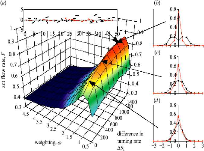
distance from trail centre (cm)
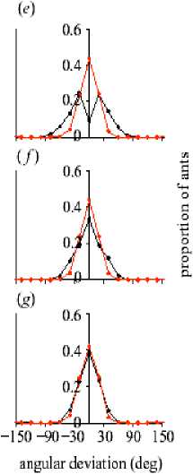
-
Figure 16. Simulation of ants on bi-directional trails
-
(a) The rate of movement of ants along a trail, F, as a function of the directional preference, ω , and asymmetry of the avoidance turning rate, θ . Inset, snapshot of the simulation in the area of parameter space where F is maximized, showing returning ants (red) tending to occupy the centre of the trail and outbound ants (black) are tending to occupy the periphery (units: cm); (b - d) Distribution of ants from the trail centre at AOa = 1400° s - 1 , 600° s - 1 and 200° s - 1 , respectively. Results calculated at t = 5000, and the means of 100 replicates shown; (e - g) Angular deviations of ants after avoidance maneuvers at A0a = 1400° s - 1 , 600° s - 1 and 200° s - 1 , respectively. Results shown are from the first 5000 interactions when t > 5000
-
The model reveals how individual ant follows chemical trails and that simple and local rules can account for the ability of army ants collectively to select a direction on a given section of trail. Furthermore, we show how an asymmetry in turning rate (during interactions with others) between outbound and returning army ants can generate a three-lane structure, in which returning ants occupy the central lane on bidirectional trails. This acts to reduce the number of high-speed collisions between ants, moving in different directions, and, consequently, increases the flow of ants to and from the nest.
The latter organization may further increase traffic flow by reducing the interface between ants moving in different directions along a trail and, hence, minimizing time-consuming head-on interactions. Such two-lane traffic flow can be simulated by incorporating a bias in turning direction during interactions, such that all ants predominantly turn either clockwise or anticlockwise. However, a two-lane structure introduces an asymmetry into the trail system, and this ‘handedness’ in the extended phenotype (swarm) is likely to limit its overall efficiency (for example by biasing the ability of ants to raid to one side or another from a central trail). Another probable reason why two lanes would not be advantageous is that returning ants are thought to deposit more pheromone than outbound ants ( Deneubourg et al. 1989). Thus, given that all ants exhibit a tendency to move towards the highest pheromone concentration, a two-lane system would not be spatially stable: outbound ants would have a tendency to drift to the side where ants return, forcing these ants further to that side, and so on.
Thermodynamics and information-theoretic measures of Agent-Based Models (ABM)
We will discuss these phenomena on agent-based modeling (ABM) examples. Modeling and simulation approaches used in ABM or computational modeling allow us to create new worlds from scratch, modifying various conditions and parameters as the need arises. ABM thus examines «emergent» behavior as a structure and pattern that develops from numerous micro-level interactions. Nonlinear dynamics, psychology, and life sciences are organized in a fashion that reflects the ability of agent-based modeling to bridge the so-called «micro-macro» divide.
In other words, ABM can be exploited to model processes at very fundamental, micro levels of analysis such as cooperation among individuals to intermediate levels such as organizational behavior in firms or other entities, all the way to «macro» phenomena such as the behavior of states or global economic processes. Therefore, we can present in a sequence that moves from more micro-level applications of ABM to increasingly macro-level applications. Two of the most micro-level analyses examine non-human systems, specifically the behavior of ant colonies and ovarian cycle variability in research rats. These examples help illustrate the highly impressive search of agent-based methodologies.
Agent-Based Models (ABM)
Agent-based modeling is based on the assumption that some phenomena can and should be modeled directly in terms of computer programs (algorithms), rather than in terms of equations. Examples arise in physical, chemical, biological and social sciences; they can be as simple as propagation of fire and simple predator-prey models between handfuls of species and as complex as the evolution of artificial societies. The central idea is to have agents that interact with one another according to prescribed rules. This type of modeling has started to compete and, in many cases, replace equation based approaches in disciplines such as ecology, traffic optimization, supply networks, and behavior-based economics. The origins of agent-based modeling can be traced to cellular automata — rows in a checkerboard that evolve into the next row based on simple rules. A physical example may be the propagation of fire in a forest. The trees may be represented as occupying a fraction of the squares in a checkerboard; the rule may be that fire propagates if two trees are adjacent via the face of a square. Thus, fire propagates though faces-up, left, and right, but not diagonally. More generally, the basic building blocks may be identical or may differ in important characteristics; moreover, these characteristics may change over time, as the agents adapt to their environment and learn from their experiences resulting in feedback (see, for example, Epstein & Axtell , 1996). A very large number of didactic and exploratory ABM’s arising in various disciplines appear in Wilenesky , 1999).
Consider, for example, a model of social segregation inspired by the work of Thomas Schelling (1978). The reader will note a similarity to the Ising model and spinodal decomposition. This model mimics the behavior of two types of individuals, reds and greens, in a city, which is represented as a checkerboard. The number of reds and greens are equal and empty spaces may be present. Reds and greens get along with each other. However, reds and greens want to live near at least some people of their own color. Initially, reds and greens are randomly distributed throughout the city. But many individuals are unhappy, since they do not have enough neighbors with the same color. Unhappy individuals move to new locations, tipping the balance of the local population, prompting others to leave. If red people move into an area then local green people might leave, and vice-versa . Over time, the number of unhappy individuals decreases. Simulations show how individual preferences propagate through the city, leading to large-scale patterns, with large clusters of red-green. For example, in the case where each individual wants at least 30% of neighbors with the same color, we end up (on average) 70% same-color neighbors. Thus, relatively weak individual preferences can lead to significant overall segregation. «The interplay of individual choices…is a complex system with collective results that bear no close relation to the individual intent», – Schelling wrote.
Some of the most challenging cases of agent-based models may be those involving economics (e.g., Epstein & Axtell , 1996). These approaches differ significantly from classical modeling systems via mathematical analysis. Classical microeconomic analysis assumes that consumers are identical and that they never change their preferences or characteristics; also, the consumers either do not communicate at all or they interact in some type of random fashion. Any inclusion of heterogeneity, organization, or adaptation would require the use of computer simulation or of numerical analysis. Applications of cellular automata to problems familiar to ChEs are those involving fluid flow and flow of granular matter (e.g., Peng & Herrmann ,
1995, 1994; Désérable , 2002). These techniques should be considered complementary rather than competitive to continuum-based and discrete-particle methods. The idea of cellular automatons can be traced to John von Neumann and Stanislaw Ulam , further developed and popularized in Conway’s Game of Life, and more recently Wolfram. It is interesting to note that Watson and Crick ’s work unraveling the structure of DNA took place nearly concurrently with much of von Neumann’s study of machine reproduction. It is noteworthy that the logical basis of reproduction in living cells mimics von Neumann’s machine reproduction theory; in fact, biology’s terminology closely follows von Neumann theory. But the converse is also true. Biology has been instrumental in driving agent-based models.
The most celebrated examples are based on the behavior of ants. In fact, ants have become the workhorse of agent-based modeling (see, Fig. 17).
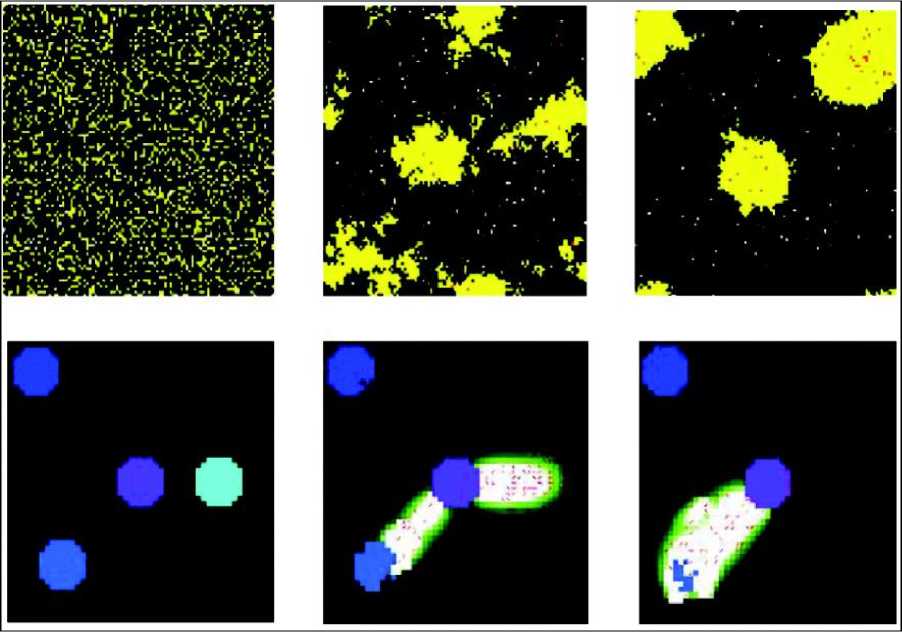
Figure 17. Agent-based models
Remark . Leftmost column in Fig. 17 shows the initial state; the two other columns show intermediates times, with time increasing left to right. Top row , termites build mounds with no central controlling authority. The algorithm is remarkably simple: each termite walks randomly. If it bumps into a wood chip, it picks the chip up, and continues to wander randomly. When it bumps into another wood chip, it finds a nearby empty space and puts its wood chip down. Bottom row , ants looking for food (a central nest and three sources of food). Ants move randomly and when they find food go back to the nest depositing a trail of pheromone. Ants tend to follow concentrated paths of pheromone, and as more ants carry food to the nest, they reinforce the chemical trail. In general the ant colony exploits the food sources in order, starting with the food closest to the nest. (Both systems can be viewed in ccl.northwestern.edu/netlogo).
Remark . ABM study exploits the analysis of insect behavior as an instance of the important overarching principle of self-organization. While self-organization is critical to the phenomenon we refer to as complex adaptive systems, the theoretical foundation of self-organization requires further study. ABM demonstrates measures of order creation and constraint production, then uses these measures to evaluate several important questions involving the nature of complex systems, including the relationship of constraints to entropyproducing processes, the role of positive feedback loops in structure formation and the extent to which constraint decay plays a role in self-organizing dynamics. The role of ABM in helping answer these questions yields some potentially crucial theoretical insights that may lead to important advances in the modeling of social behavior.
Ants have the ability to find the shortest path to food sources without using any visual cues. This much is known: Ants deposit pheromones while walking and ants prefer to follow directions rich in pheromone. Also, pheromone diffuses and evaporates, that is, trails do not last forever. These facts explain how ants can find the shortest path if a trail is broken and an obstacle disrupts the trail. The ants that pick the shorter path around the obstacle reconnect more quickly to the interrupted pheromone trail than those that choose the longer path. The pheromone scent is stronger in the shortest path; it gets picked, and over time reinforced. Thus, finding the shortest path around the obstacle emerges as a property of the interaction between the obstacle shape and the ants’ distributed behavior. The same mechanisms help ants to pick the closest source of foods.
Can ants be used in practical situations?
The answer is yes .
Consider the Traveling Salesman Problem (TSP). Say, for example, that salesmen have to visit ten cities, and that takes different times to travel between any two of them. What is the shortest path where each city is visited once? Consider now that an army of virtual salesmen (ants) are released to explore, randomly, all possible routes in the map. After an ant successfully completes the trip, it traces back the path to the original city, depositing an amount of virtual pheromone along the path. After the first round of explorers, a new batch is released and instructed in some way to follow the most concentrated routes. Because of diffusion and evaporation, the concentration is lower on longer paths. With tens of thousands of ants exploring the map and seeking high concentration routes, short routes accumulate higher concentrations, while long and convoluted routes accumulate almost no pheromone at all. The process is autocatalytic. After several repetitions, the shorter routes are reinforced reaching a near-optimal path. This is precisely the SI approach devised by Marco Dorigo ( see Bonabeau et al., 2000). The method leads to solutions that appear to be better than the Shortest Path routine used by the Internet to find paths between nodes of the network.
-
A . Ants and Near-Optimal Paths applications. Thus ants have the ability to calculate the shortest path to different food sources using trails of pheromone. Replace sources of foods with cities and ants with salesmen: this analogy leads to a new way to view the classical TSP. Ant-inspired simulations developed in the late 1990s have led to algorithms that find near-optimal routes in networks. France Telecom, MCI, and British Telecommunications have used antlike routing strategies to telephone and data networks ( Bonabeu et al., 2000).
-
B . Emergent patterns in multi-agent communication space: information-theoretic measures on microlevel. Self-organization may seem to contradict the second law of thermodynamics that captures the tendency of systems to disorder. The «paradox» has been explained in terms of multiple coupled levels of dynamic activity – the Kugler-Turvey model ( Kugler and Turvey , 1987) – self-organization and the loss of entropy occurs at the macro-level, while the system dynamics on the micro-level generates increasing disorder. One convincing example is described by Parunak and Brueckner (2001) in the context of pheromone-based coordination. Their work defines a way to measure entropy at the macro level (agents' behaviors lead to orderly spatiotemporal patterns) and micro level (chaotic diffusion of pheromone molecules). In other words, the micro level serves as an entropy «sink» – it permits the overall system entropy to increase, while allowing self-organization to emerge and manifest itself as coordinated multi-agent activity on the macro level. Another example relates a macro-level increase of coordination potential within a multi-agent team, indicated by a macro-level decrease in epistemic entropy of agents' joint beliefs, with a micro-level increase in the entropy of the multi-agent communication space ( Prokopenko and Wang , 2004).
Similarly, it can be shown that the emergence of multi-agent networks, indicated by the minimal variance of their fragments (an approximation of the network heterogeneity), is explained by increased entropy on a micro-level. This micro-level is the communication space where the inter-agent messages are exchanged (Prokopenko et al., 2005). A characterization of the micro-level (the entropy «sink») can be obtained if one estimates the «regularity» of the communication space. The auto-correlation function is equivalent to the power spectrum in terms of identifying regular patterns – a near-zero auto-correlation across a range of delays would indicate high irregularity, while auto-correlation with values close to one indicate very high regularity. Another useful regularity statistics (based on the correlation dimension) is given by approximate entropy (ApEn) that quantifies the unpredictability of fluctuations in a time series as the likelihood that «simi-lar» patterns of observations will not be followed by additional «similar» observations (Pincus, 1991). In other words, a time series containing many repetitive patterns has a relatively small ApEn, while a more complex series has a higher ApEn. In summary, macro-level («global-view») metrics may capture the quality of the emergent solutions in terms of observable coordination activities, while micro-level metrics may verify the solution in terms of the multi-agent communications.
-
C . Self-organization in multi-agent systems and thermodynamic concepts . To be effective, multi-agent systems must yield coordinated behavior from individually autonomous actions. Concepts from thermodynamics (in particular, the Second Law and entropy) have been invoked metaphorically to explain the conditions under which coordination can emerge. Emergent self-organization in multi-agent systems appears to contradict the second law of thermodynamics. This paradox has been explained in terms of a coupling between the macro level that hosts self-organization (and an apparent reduction in entropy), and the micro level (where random processes greatly increase entropy). Metaphorically, the micro level serves as an entropy «sink», permitting overall system entropy to increase while sequestering this increase from the interactions where self-organization is desired. This metaphor make precise by constructing a simple example of pheromone-based coordination, defining a way to measure the Shannon entropy at the macro (agent) and micro (pheromone) levels, and exhibiting an entropy-based view of the coordination.
Self-organization in natural systems (e.g., human culture, insect colonies) is an existence proof that individual autonomy is not incompatible with global order. However, widespread human experience warns us that building systems that exhibit both individual autonomy and global order is not trivial. The relation between self-organization in multi-agent systems and thermodynamic concepts such as the second law is not just a loose metaphor, but can provide quantitative, analytical guidelines for designing and operating agent systems.
Remark . The experience is sometimes summarized informally as «Murphy’s Law», the observation that anything that can go wrong will go wrong and at the worst possible moment. At the root of the ubiquity of disorganizing tendencies is the Second Law of Thermodynamics that «energy spontaneously tends to flow». In the context of biomechanical systems, Kugler and Turvey (1987) suggest that self-organization can be reconciled with second-law tendencies if a system includes multiple coupled levels of dynamic activity. Purposeful, self-organizing behavior occurs at the macro level. By itself, such behavior would be contrary to the second law. However, the system includes a micro level whose dynamics generate increasing disorder. Thus the system as a whole is increasingly disordered over time. Crucially, the behavior of elements at the macro level is coupled to the micro level dynamics.
State, and thus entropy, can define in terms either of location or direction. Location-based state is based on a single snapshot of the system, while direction-based state is based on how the system has changed between successive snapshots. Each approach has an associated griddling technique. For location-based entropy, the field with a grid is divided.
Fig. 18 shows a 2 x 2 grid with four cells, one spanning each quarter of the field (H. Parunak, & S. Brueckner, « Entropy and self-organization in multi-agent systems» , Proc. of the Fifth International Conference on Autonomous Agents , Montreal: ACM Press, 2001, pp. 124-130).
The state of this system is a four-element vector reporting the number of molecules in each cell (in the example, reading row-wise from upper left, < 1, 1, 3, 2 >. The number of possible states in an n x n grid with m particles is n 2 m . The parameters in location-based gridding are the number of divisions in each direction, their orientation, and the origin of the grid.
For direction-based entropy, we center a star on the previous location of each particle and record the sector of the star into which the particle is found at the current step.
Fig. 19 shows a four-rayed star with a two particles. The state of the system is a vector with one element for each particle in some canonical order. Counting sectors clockwise from the upper left, the state of this example is < 2, 3 >. The number of possible states with an n pointed star and m particles is m • n . The parameters in direction based gridding are the number of rays in the star and the rotation of the star about its center.
In both techniques, the analysis depends critically on the resolution of the grid (the parameter n ) and its origin and orientation (for location) or rotation (for direction).
Figure 18. Location-based gridding
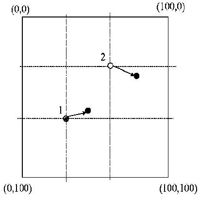
Figure 19. Direction-based gridding
Fig. 20 shows location entropy in the micro system (the pheromone molecules), computed from a 5 x 5 grid.
Figure 20. Micro entropy in time ( 5 x 5 grid)
Figure 21. Unguided walker locational entropy ( 15 x 15 grid)
Entropy increases with time until it saturates at 1. The more molecules enter the system and the more they disperse throughout the field, the higher the entropy grows. Increasing the grid resolution has no effect on the shape of this increase, but reduces the time to saturation, because the molecules must spread out from a single location and the finer the grid, the sooner they can generate a large number of different states. Directional entropy also increases with time to saturation. This result (not plotted) can be derived analytically. The molecule population increases linearly with time until molecules start reaching the edge. Then the growth slows, and eventually reaches 0.
Let M be the population of the field at equilibrium, and consider all M molecules being located at (50, 50) through the entire run. Initially, all are stationary, and each time step one additional molecule is activated. Then the total number of possible system states for a 4-star is 4 M , but the number actually sampled during the period of linear population growth is 4 t , since the stationary molecules do not generate any additional states.
Thus the entropy during the linear phase is log (4 t ) / log (4 M ). As the growth becomes sub-linear, the entropy asymptotically approaches 1, as with locational entropy. With no coupling to the micro field, the walker is just a single molecule executing a random walk.
Fig. 21 shows that locational entropy for this walker increases over time, reflecting the increased number of cells accessible to the walker as its random walk takes it farther from its base. The grid size (15 divisions in each direction) is chosen on the basis of observations of the guided walker, discussed below.
Now we provide the walker with a micro field by emitting pheromone molecules from the target.
Because of their initial random walk around their origin, walkers in different runs will be at different locations when they start to move, and will follow slightly different paths to the target.
The dots in Fig. 22 and Fig. 23 show the directional and locational entropies across this ensemble of guided walkers as a function of time.
The solid line in each case plots the normalized median distance from the walkers to the target (actual maximum 28), while the dashed line plots the normalized median number of molecules visible to the walkers (actual maximum 151). The lines show how changes in entropy and reduction in distance to the target are correlated with the number of molecules that the walker senses at any given moment. At the beginning and end of the run, when the walkers are wandering without guidance, directional entropy is 1, corresponding to a random walk. During the middle portion of the run, when the walker is receiving useful guidance from the micro level, the entropy drops dramatically. As the temperature parameter T is increased in the range 50 to 100, the bottom of the entropy well rises, but the overall shape remains the same (plot not shown).

Figure 22. Guided walker
Figure 23. Guided walker
dots - directional entropy (4 star); solid line -median distance to target (max 28); dashed line - median visible molecules (max 151)
dots - locational entropy ( 15 x 15 grid), solid line -median distance to target (max 28), dashed line -median visible molecules (max 151)
The locational entropy presents a different story. The minimization method for avoiding discreteness artifacts has the effect of selecting at each time step the offset that best centers the cells on the walkers. At the beginning of the run and again at the end, most walkers are close together, and fall within the same cell (because we chose a cell size comparable to these clouds). Walkers leave the starting cloud at different times, since those closer to the target sense the pheromones sooner, and follow different paths, depending on where they were when the pheromone reached them. Thus they spread out during this movement phase, and cluster together again once they reach the target. The effect of raising T to 100 on locational entropy is that the right end of the curve rises until the curve assumes a similar shape (plot not shown) to Fig. 20.
Comparison of Fig. 20 and Fig. 23 shows that though the directed portion of the walker’s movement has higher entropy than the undirected portions, coupling the walker to the micro level does reduce the walker’s overall entropy. Even at its maximum, the entropy of the guided walker is much lower than that of the random one, demonstrating the basic dynamics of the Kugler-Turvey model. The different behavior of locational and directional entropy is instructive.
Which is more orderly: a randomly moving walker or one guided by pheromones?
The expected location of a random walker is stationary (though with a non-zero variance), while that of a guided walker is non-stationary. In terms of location, the random walker is thus more regular, and the location entropy reflects this. However, the movement of the guided walker is more orderly than that of the random walker, and this difference is reflected in the directional entropy. This difference highlights the importance of paying attention to dynamical aspects of agent behavior. The intuition that the guided walker is more orderly than the random one is really an intuition about the movement of this walker, not its location. Let us consider one of applied example in robotics.
Swarm robotic system and snake-bot
We are focuses on a particular swarm robotic system (referred to as «swarm-bot») which is composed of a number of individual robots (referred to as «s-bots») that are assembled to each other through physical links [14, 15], and on snake-bot model. A swarm-bot can efficiently move only if the chassis of the assembled s-bots have the same orientation. A modular limbless, wheel less snake-like robot (Snakebot) without sensors is based on a novel information-theoretic measure of spatiotemporal coordination in a modular robotic system, and uses it as a fitness function in evolving the system. This approach exemplifies a new methodology formalizing co-evolution in multi-agent adaptive systems: information-driven evolutionary design.
-
A . Swarm robotic system . As a consequence, the s-bots should be capable of negotiating a common direction of movement and then compensating possible misalignments that originate during motion. At the beginning of a trial, the s-bots start with their chassis oriented in a random direction. Their goal is to choose a common direction of motion on the basis of the only information provided by their traction sensor, and then to move as far as possible from the starting position. The group is not driven by a centralized controller (i.e., the control is distributed), nor can the s-bots directly communicate or coordinate on the basis of synchronizing signals. Moreover, s-bots cannot use any type of landmark in the environment, such as light sources, or exploit predefined hierarchies between them to coordinate (i.e., there are no «leader robots» that decide and communicate to the other robots the direction of motion of the whole group). Finally, the s-bots do not have a predefined trajectory to follow, nor they are aware of their relative positions or about the structure of the swarm-bot in which they are assembled. As a consequence, the common direction of motion of the group should emerge as the result of a self-organizing process based on local interactions, which are shaped as traction forces. The problem of designing a controller capable of producing such a self-organized coordination is tackled using neural networks synthesized by artificial evolution.
Each s-bot is provided with different types of sensors, motors, and connecting apparatuses that allow groups of s-bots to self-assemble and disassemble. A swarm-bot consisting of several connected s-bots should move as a whole and reconfigure its shape when needed. For example, it might have to change its shape in order to go through a narrow passage or overcome an obstacle [15]. Thus, swarm-bots combine the power of swarm intelligence, as they are based on the emergent collective intelligence of groups of robots, and the flexibility of self-reconfiguration as they might dynamically change their structure to match environmental variability [14].
We will focus on a particular problem for the swarm-bot: coordinated motion . The s-bots are physically connected in a swarm-bot and have to coordinate their individual actions in order to move coherently. Coordinated motion is well studied in biology as it is present in many different animal species. Examples of this behavior can be seen in flocks of birds flying in a coordinated fashion, or in schools of fish swimming in perfect unison. These examples are not only fascinating for the charming patterns they create, but they also represent interesting instances of self-organizing behaviors. In [14, 15] shows how coordinated motion of real physically linked robots can be achieved on the basis of simple and robust controllers that have access only to local sensory information. In order to understand the functioning of the controller at the individual level, the activation of the motor units of an s-bot were measured in correspondence to a traction force whose angle and intensity were systematically varied.
The results are reported in Fig. 24 and Fig. 25. They indicate that at the individual level, each s-bot exhibits two tendencies: one consists in following the rest of the group (e.g., when the perceived traction comes from the left or right hand side) and the other consists in persevering in moving straight (e.g., when the perceived traction comes from the rear or from the front, or has a low intensity). The effects of the individual behavior at the group level can be described as follows. At the beginning of each test, all s-bots perceive traction forces with low intensity, and so they move forward at maximum speed (according to point 1, Fig. 25). The different traction forces generated by these movements are physically summed up by the turret of each robot. This causes a unique force to emerge at the group level, which has a direction that characterizes the movement of the whole group. The s-bots that have small misalignments with respect to this average group’s motion direction perceive traction forces from the rear and so they tend to persevere in their motion (according to point 3).
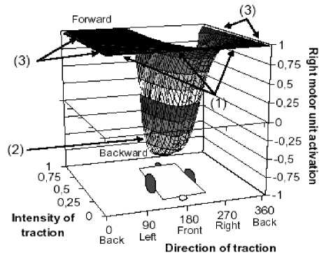
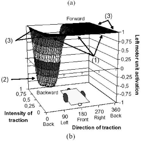
Figure 24. Motor commands issued by the left (a) and right (b) motor units
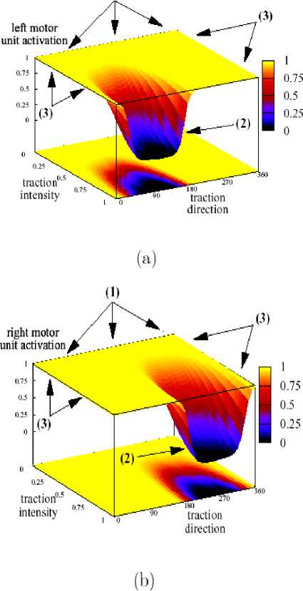
Figure 25. Motor commands issued by the left (a) and right (b) motor units
[mapped onto a [-1, 1] interval (-1 and +1 respectively correspond to maximum backward and forward speed), of one of the best evolved neural controllers in correspondence to traction forces having different directions and intensities]
[(0 corresponds to maximum backward speed and 1 to maximum forward speed), of the best evolved neural controller in correspondence to traction forces having different directions and intensities]
This simple behavioral strategy is robust. In some cases, however, the same strategy does not lead the s-bots to converge toward a common direction of motion, but rather to a rotational dynamic equilibrium in which all s-bots move around the center of mass of the swarm-bot.
This rotational equilibrium is stable since, while turning in circle, the s-bots perceive a traction force toward the group’s center that keeps them moving by slightly turning toward it. This rotational equilibrium is never observed in the experimental conditions used to evolve the controller, involving four simulated s-bots forming a linear structure, but only in generalization tests performed with real robots in different situations. In other words, the ability for a group of s-bots to display coordinated motion is the result of two opposite tendencies at the individual level: one corresponds to follow the rest of the group (e.g., when the perceived traction is not aligned with the current direction of motion) and the other to persevere in moving straight (e.g., when the perceived traction is opposite with respect to the current direction of motion, or when it has a low intensity).
Remark . Above was described the results in swarm robotics which also implements standard selfreconfigurability with task-dependent cooperation. Small autonomous mobile robots (s-bots) aggregate into specific shapes enabling the collective structure (a swarm-bot) to perform functions beyond capabilities of a single module. The swarm-bot forms as a result of self-organization «rather than via a global template and is expected to move as a whole and reconfigure along the way when needed» [14].
One of basic ability of s-bot is coordinated motion emerging when the constituent independently-controlled modules coordinate their actions in choosing a common direction of motion. The focus in this research is on how much locomotion can be «patterned» in an aggregated structure.
-
B . Snakebot model . In this section we present also experimental results of Snakebot’s evolution based on estimates of the excess entropy and the relative excess entropy [16, 17]. The Genetic Programming (GP) techniques employed in the evolution are described elsewhere. In particular, the genotype is associated with two algebraic expressions, which represent the temporal patterns of desired turning angles of both the horizontal and vertical actuators of each morphological segment. Because locomotion gaits, by definition, are periodical, we include the periodic functions sin and cos in the function set of GP in addition to the basic algebraic functions. The selection is based on a binary tournament with selection ratio of 0.1 and reproduction ratio of 0.9. The mutation operator is the random sub-tree mutation with ratio of 0.01. Snakebots evolve within a population of 200 individuals, and the best performers are selected according to the excess entropy values, over a number of generations.
Figs 26 and 27 are contrast (for vertical actuators) actual angles used by the first offspring and the final generation.
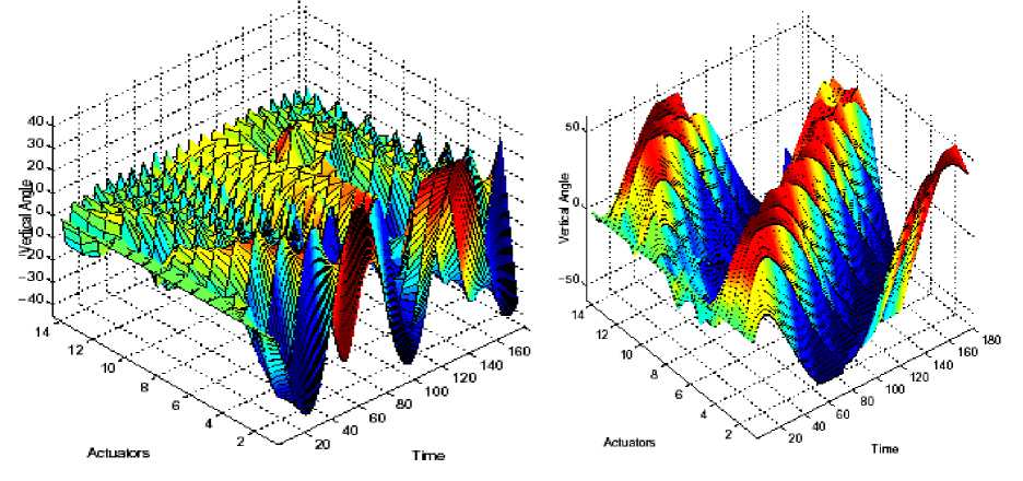
Figure 27. Evolved solution: actuator angles
Figure 26. First offspring: actuator angles
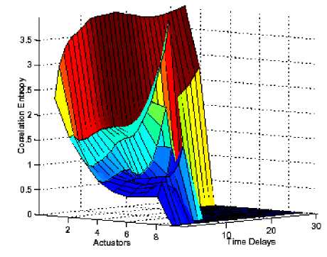
Figure 28. First offspring (correlation entropy)
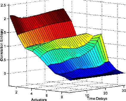
Figure 29. Evolved solution
Similarly, Figs 28 and 29 are contrasting the spatiotemporal correlation entropies produced by the first offspring and the evolved solution [16].
It can be easily observed that more regular angle dynamics of the evolved solution manifests itself as more significant excess entropy.
Figs 30 and 31 are show typical fitness growth towards higher excess entropies estimated and the relative excess entropies, for two different experiments [16].
It should be noted that there are well-coordinated Snakebots which are moving not as quickly as the Snakebots evolved according to the direct velocity-based measure, i.e. the set of fast solutions is contained within the set of well-coordinated solutions.
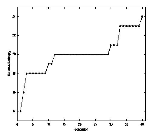
Figure 30. Snakebot fitness over time (using excess entropy)
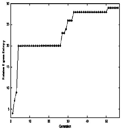
Figure 31. Snakebot fitness over time (using relative excess entropy)
This means that the obtained approximation of the direct fitness function by the information-theoretic selection pressure towards regularity is sound but not complete.
In certain circumstances, a fitness function rewarding coordination may be more suitable than a direct velocity-based measure: a Snakebot trapped by obstacles may need to employ a locomotion gait with highly coordinated actuators but near-zero absolute velocity. In fact, the obtained solutions exhibit reasonable robustness to challenging terrains, trading-off some velocity for resilience to obstacles. In particular, the evolved Snakebot is able to traverse ragged terrains with obstacles three times as high as the segment diame- ter, move through a narrow corridor (only twice as wide as the segment diameter), and overcome various extended barriers. In addition, the Snakebot is robust to failures of individual segments: e.g., it is able to move even when every third segment is completely incapacitated, albeit with only a half of the normal speed. Interestingly enough, the relative excess entropy is increased in partially damaged Snakebots, as the amount of transferred information in the coupled locomotion has to increase.
Moreover, there appears to be a strong correlation between the number of damaged (evenly spread) segments and the resulting relative excess entropy, where the coefficient of the linear fit is approximately equal to the relative excess entropy of a non-damaged Snakebot.
This observation opens a way for Snakebot’s self-diagnostics and adaptation: the run-time value of the relative excess entropies may identify the number of damaged segments, enabling a more appropriate response.
Entropy in the Overall System
Central to the Kugler-Turvey model is the assertion that entropy increase at the micro level is sufficient to ensure entropy increase in the overall system even in the presence of self-organization and concomitant entropy reduction at the micro level. The experiment illustrates this dynamic. As illustrated in Fig. 22, by time 60, normalized entropy in the micro system has reached the maximum level of 1, indicating that each of the 30 replications of the experiment results in a distinct state. If each replication is already distinct on the basis of the locations of the pheromone molecules alone, adding additional state elements (such as the location of the walker) cannot cause two replications to become the same. Thus by time 60 the normalized entropy of the entire system must also be at a maximum. In particular, decreases in macro entropy, such as the decrease in locational entropy from time 80 to 250 on seen in Fig. 23, do not reduce the entropy of the overall system. One may ask whether the reduction in macro (walker) entropy is causally related to the increase in micro entropy, or just coincidental. After all, a static gradient of pheromone molecules would guide the walker to the target just as effectively, but would be identical in every run, and so exhibit zero entropy. This argument neglects whatever process generates the static gradient in the first place. An intelligent observer could produce the gradient, but then the behavior of the system would hardly be «self-organizing».
In this scenario, the gradient emerges as a natural consequence of a completely random process, the random walk of the pheromone molecules emerging from the target. The gradient can then reduce the entropy of a walker at the macro level, but the price paid for this entropy reduction is the increase in entropy generated by the random process that produces and maintains the gradient. One may also ask whether our hypothesis requires a quantitative relation between entropy loss at the macro level and entropy gain at the micro level. A strict entropy balance is not required; the micro level might generate more entropy than the macro level loses. In operational terms, the system may have a greater capacity for coordination than a particular instantiation exploits. What is required is that the entropy increase at the micro level be sufficient to cover the decrease at the macro level.
Thus three claims of interest are:
-
1. Constraints can be constructed from entropy-producing processes in the bootstrapping phase of selforganizing systems;
-
2. Positive feedback loops are critical in the structure formation phase ;
-
3. Constraints tend to decay. The continued presence of far from-equilibrium boundary conditions are required to reinforce constraints in the maintenance phase .
These three points relate to how systems may learn the structure of their environment. As will be demonstrated, learning can be measured as an increase of constraints that limit degrees of freedom of agents ( Kugler, P. N. & Turvey, M. T., Information, natural law, and the self-assembly of rhythmic movement . Hillsdale, NJ: Lawrence Erlbaum , 1987). Specifically, learning in agent-based model (ABM) can occur through (a) changes in agent interaction patterns e.g. edge weighting in neural networks ( Rumelhart & McClelland , 1986), (b) changes in agents’ internal rules, e.g. distributed classifier systems ( Holland , 1995) or (c) changes to potential information stored in the environment, e.g. pheromone trail following in ant foraging systems (Bonabeau, Dorigo & Theraulaz, 1999).
The discussed model uses this last, stigmergic form of learning. However, these principles should equally apply to the first two forms of learning. The following simulation of food gathering ants is presented for the purpose of calculating statistical and thermodynamic measures that help characterize phases of selforganization.
The ant system described here is discrete; the positions of all objects in the system are specified by a 2tuple of integers ( x , y ). The space of positions is a square grid. The three types of objects are nests, food, and ants. Ants and the environment are modeled as active agents in the simulation. Additionally, each position in the space can contain some amount of nest pheromone and food pheromone, which are deposited by the ants as they move.
A basic simulation is set up as follows: A nest and some amount of food are placed in the space. A fixed number of ants is initially placed at the nest. All positions have zero levels of both food and nest pheromones. The system evolves as the ants move, drop pheromone, and transport food. The model is flexible to later allow experimentation of initially placing ants at any location in the space and to allow any type of object (nests, food, ants) to be introduced at any time or position.
Emergence of Thermodynamic Constraint in Self-organizing Systems
Three claims from non-equilibrium thermodynamics were explored in the context of an ant foraging agent-based model: (1) Constraints can be constructed from entropy-producing processes, (2) Positive feedback loops are critical to structure formation, and (3) The continued presence of far-from-equilibrium boundary conditions are required to reinforce internal constraints.
Measures of constraint and order that illustrate these claims are developed. These initial findings can be considered first steps in establishing mappings from non-equilibrium thermodynamics to ABM. To consider non-physical representations of work, one can enumerate the degrees of freedom that characterize an agent’s behavioral repertoire. In the ant model, an ant can potentially move to 8 neighboring spaces. Degrees of freedom are removed as an ant is informed by a pheromone gradient. As the ant movement is constrained by the pheromone field, we propose the idea that work is being done on the ant by the ant-pheromone field interaction.
Fig. 32 depicts four phases of the typical evolution of the ant foraging model.
It is an extension of the work of Guerin and Kunkle (S. Guerin and D. Kunkle, « Emergence of Constraint in Self-organizing Systems», Nonlinear Dynamics, Psychology, and Life Sciences, 2004, Vol. 8, No. 2, pp. 131 – 146) in which a simple agent-based model was constructed and the processes leading to structure formation, structure maintenance, and structure decay were studied. It was found that these three features – commonly observed in complex system agent-based models – could be explained in terms of ideas from equilibrium and non-equilibrium thermodynamics. For example, when a system forms an organization, it appears to move from a state of high disorder, or, in thermodynamic terms, high entropy, to a state of low entropy.
The second law of thermodynamics contradicts such a change in an isolated system, and, in the simple ant system, it was observed that an initial increase in entropy might account for the eventual drop in entropy. Such increases in entropy, which enable the formation of organization, are the mainstay of non-equilibrium thermodynamics ( Atkins , 1984; Prigogine , 1962, 1984; Haken , 2000; and Schneider and Kay , 1995; Swenson and Turvey , 1992). Measures of constraint and spatial entropy are defined as tools for examining the construction and destruction of constraints in this self-organizing system.
The ant model will currently be used for three purposes: (1) Exploring the parameter space of the model and produce a set of phase diagrams to show how its behavior changes with differing parameter values; (2) Introducing the concept of useful work done by the system and show how this is affected by changes in the behavioral rules and initial conditions of the model; (3) Discussing the work done by the system in the language of statistical thermodynamics.
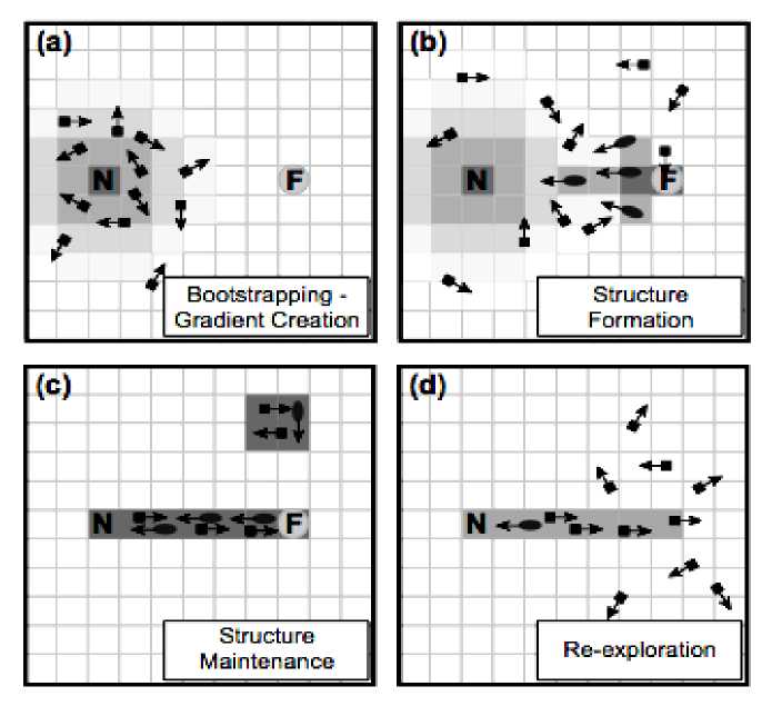
Figure 32. Typical evolution of the ant system
-
(a) Bootstrapping – Gradient Creation: Ants move randomly out from the nest, creating a gradient of nest pheromones; (b) Structure Formation: Some ants find the food and begin following the nest pheromones while dropping food pheromones that food-seeking ants begin to follow; (c) Structure Maintenance: A stable path of both food and nest pheromones is established. As shown in the upper-right corner, cycles that do not transport food can also form; (d) Re-exploration: Once all of the food has been transported to the nest the pheromones begin to evaporate and the ants disperse
-
A . Experimental Setup. The spirit of this model is an extension of the work of Parunak and Brueckner (2001), Kugler and Turvey (1987) and Gutowitz (1993). The following simulation of food gathering ants is presented for the purpose of calculating statistical and thermodynamic measures that help characterize phases of self-organization. The ant system described here is discrete; the positions of all objects in the system are specified by a 2-tuple of integers ( x , y ). The space of positions is a square grid. The three types of objects are nests, food, and ants. Ants and the environment are modeled as active agents in the simulation. Additionally, each position in the space can contain some amount of nest pheromone and food pheromone, which are deposited by the ants as they move.
-
Therefore, a basic simulation is set up as follows: A nest and some amount of food are placed in a space. All locations have zero levels of both food and nest pheromones. A conserved number of ants is placed in the system with varied spatial distributions. The system evolves as the ants move, drop pheromone, and transport food. An ant can hold one unit of food at a time and can take one of three actions: (1) move to one of eight adjacent locations (includes diagonal moves); (2) pick up a unit of food; and (3) drop a unit of food at a nest. At each time step some percentage of the pheromone present at each position «evaporates», or is removed. Also, each time step some percentage of the pheromone present at each position «evaporates», or is removed. Pheromone evaporation allows adaptation to changes in food location. For example, if there were two food sources present, A and B , and the ants were exploiting A for a period of time a strong trail of pheromones would be laid between the nest and A . Once the food at A is gone the ants should no longer follow that trail, but should rather explore again to find B . If the pheromones leading to A do not evaporate this cannot occur.
The decay or forgetting of constructed constraints (pheromone trails) allows the system to be adaptive. In some experiments, ants have directionality – they can only travel to their forward five positions instead of choosing from all eight adjacent positions (see, Fig. 33).
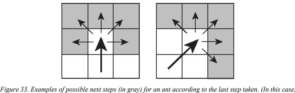
ants have fixed context-free constraints preventing backwards movement)
This local directionality – present regardless of the state of the system – is an example of a context-free constraint (Juarrero, 1999).
The direction of an ant is calculated after each step based on the previous and current positions. At time zero each ant chooses a random direction. In addition to this directionality, ants are given a behavior, in some experiments, that turns them around when they reach their goal – either the food-source or the nest. In the main set of experiments performed for this section, the turnaround behavior and the ant directionality are successively turned off to observe the result on the ant-pheromone structure formed when the system reaches a steady state. The turnaround and directionality behaviors were originally included to make the system more efficient at reaching a structured steady state, but these behaviors constitute information about the environment and it is central to this section to observe the macroscopic effect of removing this information from the microscopic actors.
Each time step, ants measure a local pheromone level then choose a direction to step. For example, for an ant with directionality, pheromone levels are read from the forward five positions. The probability of moving to position j is given by:
pj =
µα j + β ∑ N µ n α + β , n = 1
where µ j is the pheromone level at position j ; α is a scaling exponent; β is a random base; and the denominator represents the total pheromone level in all possible next positions. In this case N is five.
The scaling exponent α increases the probability that the next position will be the one with the greatest pheromone level, whereas the random base β has the opposite effect. Typical values used in our experiments were α = 3, β = 1, and a maximum pheromone level of 511 at any one position. These parameters can be adjusted to tune the likelihood that an ant will explore for new food versus exploiting a found food source. The parameter β might be thought of as a temperature. By analogy to a physical system, when the temperature is high, each particle is highly agitated and the randomness of its motion is high. Any forces – e.g. electrostatic or gravitational – have to compete with this agitation for influence over the motion of the particles. The β parameter effectively acts in the same way: high values of β can randomize the motion of the ants even in strong pheromone fields. These parameters can be adjusted to tune the likelihood that an ant will explore for new food versus exploiting a found food source. So, the movement of an ant is constrained by a measure of change not an absolute strength. One can think of the gradient as the spatial first derivative of the pheromone field.
-
B . Constraint and Spatial Entropy Measures . It is in the initial conditions and the relevant behavioral rules of the ants and pheromones that we find the propensity of the system to organize into structure. As a system organizes, either through mechanisms of self-organization or through intervention by an external designer, components of the system are expected to lose degrees of freedom through the emergence of contextsensitive constraints (Juarrero, 1999). In this system, ants lose directional degrees of freedom as they are informed by a gradient. This constraint in the model Is measured with a directional entropy. An ant that sees no pheromone gradient, which is an equal level of pheromone in all possible next positions, is said to be maximally ignorant and has an ignorance level of 1. An ant that has no choice but to move to one specific position on the next step would have an ignorance of 0, though this never occurs here because of the random base
added to each pheromone level as described in Eq. (1). In this system, work is performed on the ants as they lose directional degrees of freedom when they are informed by the pheromone field. We measure this constraint in our model with a directional entropy. An ant that sees no pheromone gradient, which is an equal level of pheromone in all possible next positions, is said to be maximally ignorant with an ignorance level of 1. An ant that is constrained to move to one specific position on the next step would have an ignorance of 0. The Shannon entropy (Shannon, 1948a, 1948b) of the probabilities of moving to each of the possible positions on the next step defines the ignorance for each ant
N
- E P n log P n
S = -n=1-------- log N where p is the probability of moving to position n, and N is the number of possible next positions, in this case five. The denominator is used to normalize the value to the range [0, 1]. The ignorance of a group of ants is defined as the average ignorance of all ants. As systems self-organize, statistical measures of order increase. In this model, we capture increased order with a spatial entropy measure applied to the positions of ants.
The spatial entropy measure is also Shannon entropy of the form shown in Eq. (2) where p is the proportion of all ants at position n , and N is the total number of positions in the space. Note that in the case of zero ants being at a location 0 • log 0 = 0 . The maximum spatial entropy is achieved with an equal number of ants at each position and the minimum with all ants at a single location.
-
C . Experimental results . The results presented here will be used to support the following three points.
-
1. In the bootstrapping phase of the ant model, an increase in spatial entropy leads to a decrease in the ignorance of the ants returning to the nest. This increase in entropy enables later phases of structure formation and maintenance.
-
2. Structure is created by a positive feedback loop of decreasing ant spatial entropy and increasing constraint (decreasing ignorance) on ant movement. A decrease in the former causes, and is caused by, an increase in the latter.
-
3. The structure is dependent on the presence of sufficient amounts of food. The presence of a separated nest and concentrated food source can be seen as a far-from-equilibrium external constraint necessary for the maintenance of structure.
These points are model-specific restatements of the three ideas from non-equilibrium thermodynamics put forth earlier. All results given here are based on an average over 20 runs with the same initial conditions. The space was 21 positions square, with a single nest at position (7, 7), a single food source at position (15,15), and all ants starting at the nest.
As an example, Fig. 34 shows the number of food seeking and nest seeking ants averaged over 20 runs of a system with 60 ants, all starting at the nest, over 500 time steps.
As would be expected, the number of each type of ant reaches equilibrium once a path between the nest and the food is established. An indicator of which phase the system is in (i.e. order parameter) could be the mean path length of the ants. The path length of an ant at a given time is defined as the number of steps it has taken since it last picked up or dropped a unit of food.
Fig. 35 shows the four phases of development with a plot of mean path length vs. time.
In the bootstrap phase the mean path length increases uniformly. The line in this case has a slope of one because each ant takes one step per unit time and no ants have yet found food. The structure formation phase begins when food is found which leads to a rapid decrease in the mean path length. During the structure maintenance phase, mean path length remains stable at a near minimum value (the shortest distance between the nest and food). When the food source is depleted, the mean path length again increases as the ants reexplore the space for alternative food sources.
Fig. 36 displays the spatial entropy and ignorance for all ants over the first 100 time steps of an experiment with an inexhaustible food source.
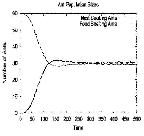
Figure 34. Relative population sizes of nest seeking and food seeking ants. As the system matures the population sizes reach equilibrium
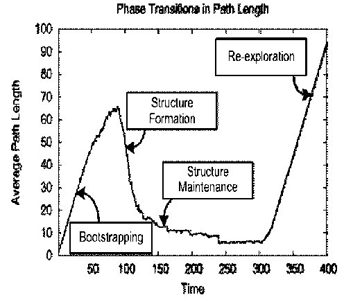
Figure 35. The four phases of development are visible in this plot of the ants’ mean path length at each time step. A path length is calculated as the number of steps an ant has taken since it last picked up or dropped a unit of food
In the bootstrapping – gradient creation phase the spatial entropy of the ants increases, which establishes a gradient of pheromones around the nest. In the structure formation phase the ignorance of the ants decreases as they find food and begin to follow the nest pheromones back. The spatial entropy of the ants also begins to decrease when a path is formed between the nest and food. The structure maintenance phase begins when the spatial entropy and ignorance of the ants becomes relatively constant.
The bootstrapping phase occurs over approximately the first 25 time steps. In this phase, the ants’ random walk from the nest causes a rapid increase in spatial entropy and the establishment of a nest pheromone gradient around the nest. In the structure formation phase ants that find food use this gradient to direct their return to the nest. The food-carrying ants’ constrained movement is reflected in a reduction of overall ant ignorance as the gradient informs them to the nest location.
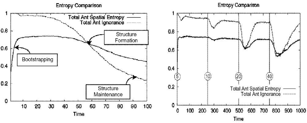
Figure 36. A comparison of the spatial entropy and ignorance of ants over time
Figure 37. Ant spatial entropy and ignorance over time as greater amounts of food are injected into the system
Increasing spatial entropy causally constraining ant movement is offered as an illustration of Point (1): Constraints can be constructed from entropy-producing processes in the bootstrapping phase of selforganizing systems. This is also in agreement with Parunak and Brueckner ’s (2001) findings (see above). They describe this effect as «coordination can arise through coupling the macro level (in which we desire agent self-organization with a concomitant decrease in entropy) to an entropy increasing process at a micro level» (p. 130).
Fig. 37 demonstrates the dependence of the structure formation and structure maintenance phases on a food source. In this case, limited amounts of food are injected every 250 time steps, starting with 5 food units at time zero and doubling the amount of food added each interval.
Remark . The vertical lines represent points at which food is injected (always at the same location). Food is injected every 250 time steps, starting with 5 food units and doubling each time. Increased order arises with larger injections of food, as shown by the more pronounced decreases in entropy.
In the presence of a concentrated food source, structure is created as shown by the decreasing spatial entropy and decreasing ignorance of the ants. Once that food source is depleted the structure breaks up as the constraints on the ants’ movements (the pheromone field) gradually decay. This effect is offered as an illustration of Point (3): Constraints tend to decay. The continued presence of far-from-equilibrium boundary conditions are required to reinforce constraints in the maintenance phase . There is a correlation between spatial entropy and ignorance in Fig. 36. This correlation is due to the positive feedback loop between decreasing ant spatial entropy and increasing constraint on ant movement (decrease in ignorance).
Fig. 38 makes this correlation (ρ=0.94) more clear with a scatter plot of ant spatial entropy vs. ignorance. A correlation coefficient of ρ=0.94 implies a link between the two. The rightmost outliers of high ignorance and low spatial entropy occur during the bootstrapping phase when ants leave the nest. The correlated points occur during the structure formation , structure maintenance , and re-exploration phases. This relationship is put forth to illustrate Point (2): Positive feedback loops are critical to structure formation. The few uncorrelated points occur during the bootstrapping phase as spatial entropy is increasing while ignorance remains at its maximum value.
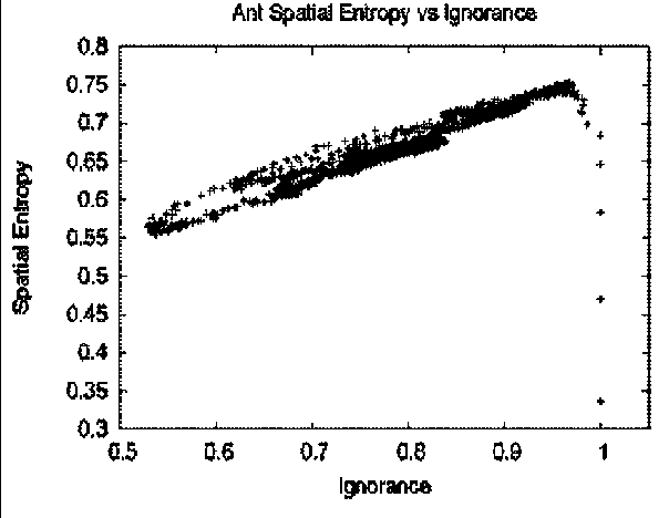
Figure 38. Plot of ant spatial entropy vs. ignorance for the experiment shown in Fig. 37
Three claims from non-equilibrium thermodynamics were explored in the context of an ant foraging agent-based model: (1) Constraints can be constructed from entropy-producing processes, (2) Positive feedback loops are critical to structure formation, and (3) The continued presence of far-from-equilibrium boundary conditions are required to reinforce internal constraints. Measures of constraint are developed and order that illustrate these claims. These initial findings can be considered first steps in establishing mappings from non-equilibrium thermodynamics to ABM.
Next steps could explore various cycles present in this model as they may relate to thermodynamic work cycles which are considered necessary for Kauffman’s Autonomous Agents (2000, 2003). Candidate cycles
Электронный журнал «Системный анализ в науке и образовании» Выпуск №3, 2014 год in this model include (i) ant movement cycles between nest and food sources, and (ii) system cycling through the phases of bootstrapping, structure formation, maintenance and re-exploration.
Remark . An Autonomous Agent ( Kauffman , 2000), in brief, is a collectively autocatalytic system performing one or more thermodynamic work cycles that: (1) measures useful displacements from equilibrium from which work can be extracted; (2) discovers devices to couple to those energy sources such that work can be extracted; and (3) applies work to develop constraints to extract further work. A primary task in examining a given organization is to understand how the system is displaced from equilibrium and how work is extracted from these initial boundary conditions. This exercise is necessarily couched in the language of thermodynamics and statistical physics. We are challenged to map this description not only to physically organizing systems, but to biological, social and computational instances of organization as well. The aim is to make the mapping without the crutch of metaphor. We will appropriate the language and methods of statistical thermodynamics through the generalization of the thermodynamic processes of heat and work for definition in non-physical systems.
Entropy
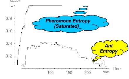
|
60 55 ■ 50 ★ 45 ■ 40 ; 35 ■ .50 - ^ДЦ^ 25 • 25 30 35 40 45 50 55 Setup |
1г p---------------=----- ° " ^-^pheromone Entropy J (Saturated)- 0.6 ■ Г ------ । г Entropy Х-/ _LL----------------------------------------------- tline 50 100 150 200 250 Where did the Entropy Go ? (a) |
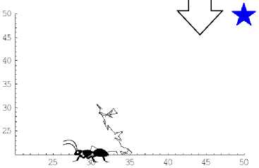
Ant Path with No Pheromones
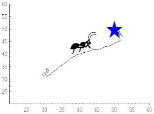
Ant Path with Pheromones
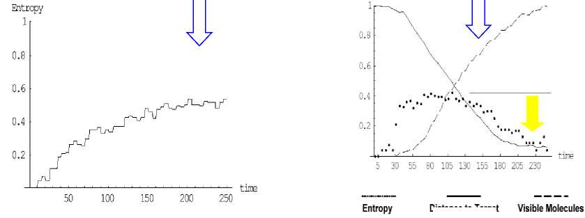
Unguided Ant’s Entropy
Distance to Target
Guided Ant’s Parameters
(b)
Figure 39. Pheromone and ant entropy (a) and quided ant’s parameters (b)
Taking guidance from Atkins (1984), we can understand heat to be the unconstrained transfer of energy and its complement, work, to be the constrained transfer of energy. More generally, we might consider heat and work to be unconstrained and constrained processes. Consider a purely physical system where work was performed to create an initial concentration of a conserved quantity (e.g. energy, mass, charge, linear momentum, angular momentum, etc.) in space. A diffusion process from thermal agitation can spontaneously arise to move the system to equilibrium absent constraint. This process of the unconstrained transfer of a conserved quantity is a heat process. Consider an alternative equivalent system comprised of a conserved quantity of computational entities (agents) performing a random walk in space. Beyond analogy, it is generally accepted that this agent system generates equivalent macroscopic dynamics that diffuse an average distance that scales with ■Jt.
Fig. 39 shows the dynamic of ant path without/with pheromone and corresponding entropy behavior.
We anticipate a theory of organization to generalize the common structuring processes present in Rayleigh-Bénard convection, lasers, cellular slime molds, immune systems, genetic regulatory networks, neural systems, and social insect systems. A robust theory should also apply to systems of more commercial interest including firms, supply webs, financial markets, transportation systems, manufacturing production lines and consumer markets. This section explores how Kauffman’s Autonomous Agent might be used as a foundation for such a theory of organization and will use the context of a familiar computational model of an ant foraging system to demonstrate how the emergence and degradation of constraints simultaneously define the process of organization.
In the ant model to be described below, the initial diffusion of random ant movement from a nest source is such a process. We describe this as a heat process in a non-physical system. Candidate cycles in this model include (1) ant movement cycles between nest and food sources, and (2) system cycling through the phases of bootstrapping, structure formation, maintenance and re-exploration.
The ants as agents have extremely simple rules of gradient-following and pheromone dropping. No individual ant is capable of learning the location of the food source. Learning and intelligence takes place in the colony – environment system taken as a whole. An idea put forth in this section is that «agent-agent» and «agent-environment» interactions along with internal rules of agents can be considered forms of constraint. From this perspective, organization can be measured, in part, as a bundle of self-reinforcing and evolving constraints.
-
D. Exploration of the parameter space of the model. With any model, it is important to know how the parameters affect the overall system behavior. In this section we look at the three main parameters governing the model: pheromone evaporation rate; number of ants; noise or «temperature» parameter β . When several model runs are averaged over, we determine the effect of varying these parameters by looking at the following metrics:
-
1. Directional entropy (defined in the previous section, Experimental Setup). Directional entropy can be considered a measure of how much work is being performed on an ant.
-
2. Mean-free-path of the ants. This is the average number of steps traveled by an ant between picking up and depositing a piece of food.
-
3. Number of food pieces picked up in a model run. The higher the number of pieces of food taken from food-source to nest over a run, the more efficient the system has become at performing this task. This is a measure of useful work performed.
A high mean-free-path value indicates that the ants are traveling large distances between picking up and depositing food; in this case, the system is unorganized – strong pheromone paths between food and nest have not yet been formed and the ants take many steps in moving between food and nest. Low values of mean free path indicate that the ants go almost directly from food to nest and back, without much deviation.
The surface plots (Figs 40–42) show the behavior of the system when the parameters are changed.
A basic summary of these results is as follows: a low pheromone evaporation rate, a large number of ants, and a low temperature are required for organization to occur. Organization is measured in the plots by: low directional entropy; low mean-free-path (whose surface plot, though absent here, is very similar to that for the directional entropy); and a high number of food pieces collected. In each case, the organized state is seen as a transition to a trough or a peak in the surface defined over the parameter space.
It can be seen that these transitions are fairly abrupt – the landscape is relatively flat but it rises or falls rapidly. We can think of these changes, from the unorganized state, as phase transitions.
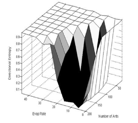
Figure 40. An exploration of the effect of evaporation rate and number-of-ant changes on the final average directional entropy of a colony
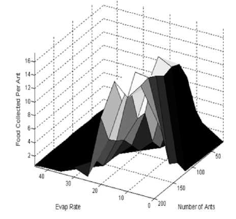
Figure 41. The effect of changing the pheromone evaporation rate and the number of ants on the total food collected per ant
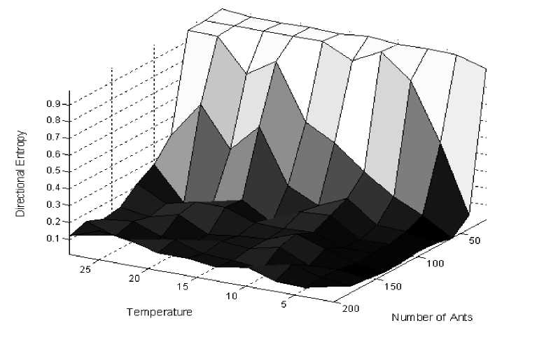
Figure 42. The effect of changing the temperature (noise parameter) and the number of ants on the average directional entropy
-
E . The effect of the behavioral rules and initial conditions on the organization formed . An interesting question to ask of a dynamical system, such as our ant model, is: what happens to the final state of the system, and its evolution to this final state, when behavioral rule changes, or changes to the initial conditions, are made? We look here at several rule settings and initial conditions. As a baseline experiment, we turn off the ant pheromone and the directionality and turnaround behavior. In this case, we have a population of 'random' ants, similar to a non-interacting gas. The ants still pick up food at the food-source and deposit it at the nest, but, along the way, they neither sense nor deposit pheromone. The baseline experiment is numbered zero; the other experiments we perform are as follows:
Rule Changes : 1) Basic ants; 2) Basic ants with directional motion; 3) Basic ants with directional motion and turnaround behavior.
Initial Condition Changes : 4) All ants begin at the nest; all are food-seeking; 5) Ants begin randomly distributed, all are food-seeking; 6) Ants begin randomly distributed (half are food-seeking; half are nestseeking).
The «basic ant» indicated above is simply an ant with no directional behavior i.e. no directional rule or turnaround behavior when the ant reaches the food or nest. The three initial condition changes are all performed for ant systems in which the ants are equipped with their full set of rules i.e. directionality and turnaround. The purpose of these experiments is to begin to understand how much information – relevant to the construction of a stable and efficient final organization – is present in the initial conditions of the ants. As we add behavioral rules to the ants, the overall number of food pieces picked up increases – the system grows in efficiency at this task.
The results for the total number of food pieces picked up are, for each experiment :
|
Exp 0 |
Exp 1 |
Exp 2 |
Exp 3 |
Exp 4 |
Exp 5 |
Exp 6 |
Exp 7 |
Exp 8 |
Exp 9 |
|
4 |
8 |
2074 |
3367 |
4046 |
455 |
980 |
336 |
4608 |
2198 |
The previous section showed evidence that when the colony is efficient at food collection, the ants have low directional entropy and mean-free-path and are organized into a tight structure. It follows, therefore, that the addition of relevant, context-dependent, rules results in the formation of a tighter colony structure and a greater potential for the system to organize to perform the task of food collection.
Changes in the initial conditions also result in striking differences in the capability of the colony to selforganize. Two factors were identified as displacements from equilibrium in our model. First, the behavioral rule that changes the ant state between food-seeking and nest-seeking after touching a nest or food patch, creates concentration gradients of differentiated ant types with reciprocal sources and sinks at the nest and food. This system partitioning occurs even as the total ant distribution remains equipartitioned in the space. The second displacement from equilibrium occurs in some experiments when ants are initially biased to be either all food-seekers and/or concentrated at the nest or food source. With all ants in their food-seeking state and beginning at the nest, the overall number of food pieces picked up is large (as expected, experiment 4) is close to experiment 3)). When the ants are initially randomly distributed, the ability of the colony to organize is significantly reduced – the total number of food pieces picked up is much smaller for experiments 5) and 6) than for 4).
Experiments 1), 5) and 6) share an interesting feature: despite the low number of food pieces picked up, the system does stabilize to a kind of structure – small clusters of ants form throughout the space. These clusters are composed of both nest- and food-seeking ants, one kind laying a pheromone trail attracting the other and, therefore, following the other. The result is a collection of tight loops and an organization that is totally inefficient at performing the task of food transportation. This loop formation is an example of useless, or pathological, self-organization.
In an attempt to investigate a rule change that might rid the system of this pathological behavior, we limit the total pheromone that each ant can deposit between visits to the food and nest. The ants are given 15 units of pheromone and can, therefore, take 15 steps before their pheromone has depleted. When a nestseeking and food-seeking and become caught in a loop, it will not be long before the pheromone of the loop is no longer reinforced and the ants move away to discover other pheromone trails. We look at the following two cases: 7) Basic ants with limited pheromone, 8) Basic ants with directional and turnaround behavior and limited pheromone.
We also look at the system for ants which have directional behavior but which, instead of encountering a 3 cell «wall» blocking their reverse path, encounter only one cell – the cell directly behind them. This softening of this constraint might be expected to result in more meandering ant behavior and, hence, less well-formed organization. Therefore, our final experiment is: 9) Basic ant with one cell directional and turnaround behavior. The number of food pieces gathered for these three experiments is as follows: 7) 336, 8) 4608, 9) 2198. The effect of limiting pheromone is to increase the effectiveness of the resulting colony at food collection – the directional entropies are also lower than for the unlimited pheromone counterparts. Experiments 7) and 8) should be compared with 1) and 3). Experiment 9) confirms our suspicion that the ants meander more when they are less constrained.
The results of the baseline experiment show that the case of no organization – the random ants are, by definition, incapable of forming structure – actually results in a greater overall amount of food picked up than the case in which ants drop and sense pheromone but they have no directionality. The reason for this is that the pheromone-sensing ants form the above-mentioned pathological organization – an organization that almost completely prevents them from performing the task of transporting food. In summary, the results show that the greater the number of structurally-relevant context free constraints the ants possess, the better the final organization is at the task of food collection and the less likely the system is to self-organize into a structure that hinders food collection. A further behavioral modification, limiting the total pheromone that can be deposited per ant, limits this «useless» self-organization.
The physical concept of quantum entanglement is brought to the biological domain. We simulate the cooperation of two insects by hypothesizing that they share a large number of quantum entangled spin-1/2 particles. Each of them makes measurements on these particles to decide whether to execute certain actions. In the first example, two ants must push a pebble, which may be too heavy for one ant. In the second example, two distant butterflies must find each other. In both examples the individuals make odor-guided random choices of possible directions, followed by a quantum decision whether to push/fly or to wait. With quantum entanglement the two ants can push the pebble up to twice as far as independent ants, and the two butterflies may need as little as half of the flight path of independent butterflies to find each other.
Quantum cooperation of two insects
A good part of the communication between the members of a species serves to coordinate their behavior in the interest of common survival. It is generally believed that this communication is governed by the laws of classical physics. Examples would be sound, vibration and direct touch, molecular signaling in the form of smell, and the wide field of behavioral expression, which is physically a method of modulating or emitting patterns of electromagnetic radiation. However, in the newly emerging branch of physics called quantum information it has become clear that many tasks requiring coordination between the actors can be achieved significantly better if the actors’ decisions are quantum entangled. The basis for this is Bell’s theorem, which proves that observational results obtained at two widely separated but quantum entangled sites can exhibit correlations whose magnitude surpasses that of any correlations conceivable by classical physical laws. Given the importance of correlated action between living systems it is worth while to investigate how quantum entanglement could be embedded beneficially in the stream of sensing, deciding and acting of individuals. In this section we do this by means of two examples.
We are discussed how much farther two cooperating ants could push a heavy pebble, and how much faster two distant butterflies could find each other (J. Summhammer, « Quantum cooperation of two Insects» , arXiv quant-ph /0503136 v2, 2005, 23 p.) Since the quantum entanglement is vulnerable in a thermal environment, the models incorporate the quantum entanglement in the behavior of the individuals in a way which enables them to solve the cooperative task even if the entanglement breaks down, although with less efficiency.
In physics, quantum entanglement (QE) is a statistical correlation between the properties measured on two or more separated particles or systems. The theory knows no upper limit on the complexity and on the number of the systems for which QE can exist. If only two particles or systems are involved, QE means that the result of a measurement done on one of them is not independent of the result of the measurement done on the other one, no matter how far they are apart. While correlations as such are not surprising, the particular aspect of QE correlations is their sheer strength, which can give the impression that each particle ’knows’ which measurement result has been obtained, or will be obtained, on the other one, so that it can ’behave’ accordingly in its own measurement. Einstein called these correlations ’spooky action at a distance’. Meanwhile, numerous experiments have shown the existence of these correlations, including tests which demonstrated that they are faster than light.
Mathematically, these correlations are outside of time and are thus instantaneous. Nevertheless, it is not possible to use QE for the transmission of information, because the individual measurement results are unpredictable. An important state, which will be used in the example with the butterflies below, is the so called singlet state. Here, the angular momenta of the two particles are always opposite to each other, so that both of them together have angular momentum zero. Symbolically, this state is written as
Iv), = I+-H-+), and called Bell state. Spin up (′+′) and spin down (′--′) are called, respectively. The angular momenta of two such particles can easily be measured along different directions, when the particles are sufficiently far apart. The possible results are then ′ + +′, ′ ----′, ′ + --′, and ′ -- +′. Quantum theory can only predict the probabili ties for these results, p, p, etc. What these probabilities look like depends on the particular physical state.
The probabilities for the possible measurement results are
( 5 ) p '+
= p
, ( 5 ) -
sin2 2

p
+-
= p ( 5 1 = — cos2
-+ 2

where α is the angle between the two chosen directions of measurement. Note that these expressions do not depend on the individual directions along which the angular momenta are measured. The time of the measurements is also not important. The particles need not be measured at the same time, and it is irrelevant which is measured first. Moreover, the distance of the particles plays no role. That is why these correlations are called nonlocal .
As a by-product of interactions, QE should be an omnipresent feature in nature. However, this would mostly be at the molecular level and below. In systems of macroscopic scale, be they inanimate or alive, one would expect that the effects of QE would quickly be lost, because any macroscopic system interacts permanently with the environment through the exchange of thermal radiation. And as soon as such interaction with systems outside the original QE occurs, the original QE gets diminished or fully destroyed. This is partly countered by the fact that, with increasing complexity of the entanglement – as would be the case in systems of many degrees of freedom, e.g. from molecules upwards – the deviation from classical physics as witnessed by violations of Bell inequalities becomes stronger. Therefore, traces of QE might be noticeable between such systems even after appreciable contact with the environment. In certain solids this has already been detected, because macroscopic properties like the behavior of the magnetic susceptibility are a proof of entanglement even at finite temperature. It has also been shown that the thermal environment does not only tend to destroy QE, but also permanently creates it by mediating between any two systems.
Therefore, it is not completely impossible that QE can exist in the biological realm. In fact, its obvious advantages may have helped to stabilize mechanisms utilizing QE under evolutionary pressure. First suggestions for a role of entanglement between animals have already been made in (B. D. Josephson and F. Pallika-ri-Viras, « Biological utilization of quantum non-locality », Found. Phys . , 1991, Vol. 21, pp. 197-207). There have also been hypotheses of quantum computations, which rely on QE, taking place in the brain. It has also been suggested that correlations found between the electroencephalograms from two different persons could be due to QE. Indeed, one can easily think of a wide range of biological processes, where QE would lead to a Darwinian advantage: Quantum entanglement could coordinate biochemical reactions in different parts of a cell, or in different parts of an organ. It could allow correlated firings of distant neurons. And – as shall be the topic here – it could coordinate the behavior of members of a species, because it requires no physical link and is independent of distance. It is also conceivable that QE correlates processes between members of different species, and even between living systems and the inanimate world. Specifically, the evolutionary advantage of quantum entanglement could consist in the following: Since quantum entanglement involves no transfer of information between the entangled parts, but produces effects over arbitrary distances as if information had been transferred, it can eliminate the need to develop further means of communication.
Nevertheless, QE is a fragile relation easily broken in the thermodynamic environment of living systems. It is therefore reasonable to expect that QE could have evolved predominantly with such tasks and processes, which can also be accomplished without QE, but which will consume less resource, like time or energy, if supported by QE.
Remark. Synchronizing distant clocks is a crucial process for telecommunications and satellite positioning systems. It is also important for high-accuracy experiments in fundamental physics, such as tests of the theory of relativity. Achieving synchronization can sometimes be the limiting factor in the accuracy of such measurements. A. Valencia et al. «Setting our watches by entanglement», Appl. Phys. Lett. 85, 2655–2657 (2004) have conducted a proof-of-principle experiment showing that quantum entanglement of photon pairs can provide a synchronization method that avoids the shortcomings of existing techniques. By sending two entangled photons (produced by shining laser light into a nonlinear optical material) down optical fibres 1.5 km long, they have been able to detect synchronized events with picosecond (10-12 s) accuracy over a distance of 3 km. For an entangled pair of particles, a measurement on one of them instantaneously determines the quantum state of the other. To use this for synchronization, the two photons are dispatched to detectors at the two ‘stations’ where the clocks are to be synchronized – say, a satellite and an Earth-based laboratory. If the clocks used to time the detection of many successive pairs are synchronized, the event timings will show the greatest number of coincidences when the records are compared. In cases of mismatch, the clocks can be altered until the detections coincide. As a classic example of cooperation, imagine a system of N excited at- oms. An atom is coupled to the ever-present electromagnetic fields, so an excited atom will spontaneously emit a photon. But if the N atoms reside at equivalent positions relative to the field, they all couple to the electromagnetic fields in the same way and cannot be distinguished by the way they interact with the field. Spontaneous emission from the atoms is then cooperative.
We want to present two such examples. They deal with the cooperation of two ants and of two butterflies, respectively. Their behavior is simulated in a numerical model, as is often done in theoretical biology. Ants and butterflies were chosen, because these small creatures sometimes show impressively coordinated achievements which make it hard to believe that solely the limited computational capacity of their nervous systems should be responsible for them. We will, however, not specify a physical or biological mechanism which carries and protects the systems within an individual which are entangled with similar systems in the other individual, although some remarks will be made in the discussion. We are here mainly interested in how QE could be embedded in the stream of sensing, decision making and acting of the individuals. We shall see that one way how QE could work is as an «inner voice», which suggests a specific action to the individual, despite a lack of sufficient information for a rational decision. In this sense it could operate like some quantum games, which help the players win even if there is no communication between them, so that some of these games exhibit properties of «pseudo telepathy».
Example : Two ants pushing a pebble . We look at two ants that must push a pebble towards a certain goal. Each ant is able to push with a force. In order to move the pebble a minimum force fmin must be applied. Clearly, if the pebble is too heavy to be moved by any of the ants alone, the two ants must push simultaneously, and they must push in similar directions. The two ants go about their task by making a series of simultaneous push attempts. However, at each push attempt each ant decides with a probability of 1/2 whether to push or to rest. This is where we will permit QE to come in. A push attempt is successful if the force applied to the pebble is larger than the required minimum. Then the pebble will move a little path length proportional to the force and in the direction of the force. In order that the two ants shall be able to exploit QE we will speculatively assume that somewhere in their nervous system they have a region which contains spin-1/2 systems, e.g., an array of atoms with a magnetic moment. And each of these spins shall be quantum mechanically entangled with exactly one such spin in the other ant, where any of these pairs shall be in the triplet state. An ant shall be able to make a quantum mechanical spin measurement on any of its spins. Somewhat anthropomorphically we can imagine the process of measurement to be a moment of introspection whose result the ant notices as a sudden urge to do this or that, depending on the outcome of the spin measurement.
Each of the pairs of spins shared by the two ants is reserved for a specific push attempt. Before a push attempt, an ant must make two decisions:
-
- Choose the direction of the push. This decision is derived from the sensory input, specifically from the odor emanating from the goal. The chosen direction shall be subject to a probability distribution. Thereby we simulate that the ants are not clever enough to keep concentrating on the task, or that they may be distracted by other sensory input, or that gusts of wind may temporarily obscure the olfactory information, etc.
-
- Decide whether to really push at this attempt, or whether to have a little rest. This decision will be made by a quantum measurement of the spin of the particle reserved for this attempt along the push direction just chosen. The ant will only push, if the result is «+». This option simulates an ant’s need to come to a decision about an action despite a general lack of sufficient information, or a general inability to come to an informed decision because of the limited capacity of its brain. These decisions are made independently by each ant and they are not communicated to the other ant. Of course, after the action, each ant could in principle obtain some information about the decisions of the other ant from the effect on the position of the pebble. We assume that this shall not influence an ant’s further strategy, because we wish to see the pure effect of the quantum correlations without communication between the partners. (Communication after the fact will be permitted in our next example with the butterflies).
This model of quantum entangled ants can be contrasted with one of two independent ants, in which the choice of direction happens exactly as in the quantum model, but the decisions of whether to push or to rest are made by each ant independently. We can still imagine these decisions to be based on spin measurements along the chosen directions. But the spins shared by the two ants will have no QE whatsoever. Then the above quantum mechanical probabilities p(t], p(t) and p(t^ will be independent of the chosen angles, and will have a constant value of 1/4. Note that, in this independent case, the ants will also be able to push the pebble towards the goal. And we can expect that, as long as the pebble is light enough to be pushed by a sin- gle ant, there should be little difference in how far the pebble gets pushed with a given number of attempts. However, as soon as the effort of both ants is needed to move the pebble, the quantum entangled ants will become superior. The reason is that especially for small differences between the choices of angles needed to move a pebble which is too heavy for a single ant – the ants will make the same decision of whether to push or to rest up to twice as often as the independent ants. Hence, the behavior of the quantum entangled ants will be more coordinated, resulting in fewer futile push attempts. Nevertheless, the behavior of a single ant which is quantum entangled with another one, will be indistinguishable from a completely independent ant.
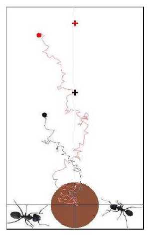
(a)
Fig. 43a shows the result of 600 push attempts of the two ants, for the independent (black) as well as for the quantum entangled case (red). It is taken from a screen shot of the simulation the actual random decisions. Ants must push the pebble to the upper line of the picture.
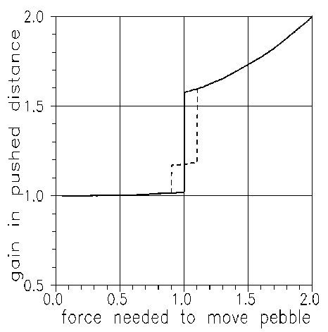
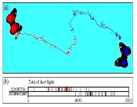
(c)
(b)
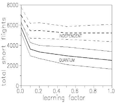
(d)
Figure 43. Typical stochastic paths of the pebble as pushed by quantum entangled ants (red) as well as by independent ants (black) (a); Gain in distance the pebble can be pushed by the quantum entangled ants relative to the independent ants, as a function of the force needed to move the pebble. Solid line: Both ants have force 1. Dashed line: One ant has force 0.9, the other has force 1.1 (b); Typical flight paths of the two butterflies. Initial distance: 1600 units. Length of one short flight: 40 units. Learning factor l = 0.5. The lines jutting out from the two main lines are short flights after which the respective butterfly had to fly back.
Note that sometimes several attempts had to be made to find a good direction (a); Statistical results of 40 independent and 40 quantum runs, respectively. Initial distance: 1600 units. Length of one short flight: 5 units. Learning factor l = 0.5. The quantum entangled butterflies needed an average of 2778 short flights to find each other. The independent butterflies needed an average of 5255 short flights (b); (c); Total number of short flights needed by the two butterflies to find each other, as a function of learning factor l. Calculated from 40 runs at each l. Solid lines: Average and range of standard deviation for quantum entangled butterflies. Dashed lines: For independent butterflies (d)
The erratic lines with the fat endpoints show typical paths of the pebble. The crosses indicate the theoretically expected endpoints of the pebble. For the sake of simplicity the probability distribution for the choice of push directions of an ant has been assumed to be the same for both ants and was taken as piecewise linear for positive and negative angles. Typical stochastic paths of the pebble as pushed by quantum entangled ants (red) as well as by independent ants (black). In both cases 600 push attempts were made.
The crosses show the theoretically expected endpoints of the pebble. The probability distribution of the push directions was set such that it was three times (as likely for the ants) to push forward than to push backward. One ant could exert a force of 0.9, the other a force of 1.1.
Fig. 43b shows the ratio of the distance the pebble can be pushed by the quantum entangled ants over the distance achievable by the independent ants with the same number of push attempts. The solid line shows the case of two equally strong ants (both can exert a pushing force of 1). Not surprisingly, the superiority of the quantum entangled ants really sets in as soon as the pebble becomes too heavy to be moved by one ant alone. If the pebble requires the maximum force of the two ants, the quantum entangled ants can push the pebble twice as far as the independent ones. The reason is that both ants must push in the same direction. Then the quantum entangled ants will either both push or both rest, while the independent ants will do so only half as often. The more general case of two ants of different strength is shown by the dashed line. A certain advantage of the quantum entangled ants sets in as soon as the force needed to move the pebble is larger than can be exerted by the weak ant (which here is 0.9), because all efforts by the weak ant alone become futile. If the pebble becomes so heavy that even the strong ant cannot move it alone, the full advantage of the quantum entangled ant’s sets in.
It is interesting to note that in both scenarios a very small advantage for the entangled ants exists also when the pebble can be moved by any of the ants alone. This is due to the fact that, even for light pebbles, there is a difference in how the pebble gets moved. E.g., for large angles between the chosen directions the forces on the pebble may almost cancel each other and the pebble will not move. Such futile attempts occur with some frequency for the independent ants. But they are rare for the quantum entangled ants.
Thus, quantum entangled ants profit from making fewer «wrong decisions».
Example : Two butterflies finding with entanglement each other . With certain kinds of butterflies it is known that a male and a female can find each other even when they are initially many kilometers apart. The usual explanation is that each butterfly emanates scent molecules to guide the other one. The huge antennas of a butterfly capture the molecules, permitting it to determine the gradient of the distribution and hence the direction of the origin of the scent. Nevertheless, one may wonder, whether for large distances the information contained in the few scent molecules is sufficient to give a butterfly a clear direction where to fly. In the present scenario we shall assume that this information will allow a butterfly only to come up with a probability distribution for the directions in which it should fly. The decision whether the butterfly will actually do a short flight in the chosen direction will come from a quantum measurement. As in the case of the ants, we assume that the two butterflies share a large number of maximally entangled pairs of spin-1/2 particles, of which each butterfly holds one particle. However, here the entangled state will be the singlet state, because we want the butterflies to get the same measurement result, if they measure their respective spins along opposite directions.
The details of the scenario are as follows:
-
(i) The intensity of the scent emanated by each butterfly drops off as 1 Ir 2 where r is the distance from the butterfly;
-
(ii) The propagation of the scent is very much faster than the speed with which the butterflies fly, so that each butterfly can notice a change of the distance of the other one with little delay as a change of intensity of the scent.
-
(iii) Each butterfly moves in a sequence of short straight flights of constant length. Before such a short flight the butterfly has to make two decisions in the following order:
-
- Choose a direction for the short flight;
-
- Decide whether to really do the short flight, or whether to have a little rest.
The first decision is resolved in the usual neuronal manner: The butterfly chooses the direction for the short flight randomly, but weighted with the probability distribution of directions which it considers appropriate in view of its experience of change of intensity of the scent in the previous short flights. In the model calculations, each butterfly can choose among 16 directions evenly spaced over 2π. In the beginning, this probability distribution is isotropic. After each short flight, the distribution is updated according to a rule which will be explained later.
The second decision comes from a quantum measurement. The butterfly measures the spin-1/2 particle designated for this short flight along the chosen direction. If the result is «+», it does the short flight, otherwise it rests until the next short flight is due.
The rule for updating the probability distribution of flight directions now looks as follows. (It is only applied, if the short flight has actually taken place. If, instead, the butterfly has taken a rest, it will retain the probability distribution from before the rest.) The butterfly measures the intensity of the scent of the other one:
-
- If the increase of the intensity, i.e. the average gradient of the scent along the short flight path, is above a certain threshold, the butterfly judges this to have been a good direction and enhances the corresponding probability weight by the factor (1+ l ). This direction is then more likely to be chosen again in one of the next short flights. The parameter l can be set between 0 and 1. When it is 0, no learning from experience occurs.
-
- If the increase of the intensity is below the threshold, the butterfly flies back, because it judges this to have been a bad direction. In addition, it reduces the probability weight of this direction by the factor ( 1 + 1 ) 1 . This direction is then less likely to be chosen again in one of the next short flights.
The threshold is taken as a certain fraction of the strongest increase of the intensity of the scent encountered in the short flights until then. Therefore, as the butterflies get closer to each other, the threshold will get higher and they will become more discriminating in judging a short flight as having been good or bad.
This quantum scenario can again be compared to a scenario of butterflies who make independent decisions. In that scenario the decision before each short flight, whether to fly or to rest, is made completely independently by the two butterflies. Each will decide randomly with a constant probability of 0.5 whether to fly or to rest.
Fig. 43c shows parts of the screenshot of the program which simulates the behavior of the two butterflies. The top picture (c) demonstrates actual tracks. The interesting result is the total number of short flights including the back flights, i.e., the total flight distance the two butterflies had to cover to meet. This is shown in the lower picture (d) which indicates the statistical results of 40 runs of independent, and of 40 runs of quantum entangled butterflies, respectively. The red pointers in the upper half indicate the number of short flights of quantum entangled butterflies, the black pointers in the lower half those of the independent butterflies. It is noticeable that the quantum entangled butterflies can find each other with much fewer short flights than the independent ones. This is because the former decide more often simultaneously to actually do the short flight, if the chosen directions happen to point roughly towards one another. This in turn, gives more often valid short flights, i.e. short flights where the increase of the scent is above the threshold so that neither of them will have to fly back. Also, it leads to a quicker adaptation of the probability distribution of flight directions to favor the current good directions. The derivation of the theoretical expression for the number of short flights needed until the encounter takes place is a laborious exercise and will not be given here.
Instead, Fig. 43d shows for 40 quantum runs and for 40 independent runs, respectively, the averages and standard deviations of the total flights needed until the butterflies meet, as a function of the learning factor l . The initial distance of the butterflies is 1600 units. The length of one short flight is 5 units. The threshold for flying back is that the butterfly does not undo a short flight if the increase of the intensity of the scent of the other butterfly was at least 60% of the strongest increase of the scent found until then. Obviously, the quantum entangled butterflies find each other faster. For a learning factor of l = 0 they need only about 83% of the short flights of the independent butterflies, and for l = 1 they need only about 48%.
It may be surprising that the quantum entangled butterflies have an advantage over the independent butterflies even for l = 0, i.e., when the butterflies don’t learn from experience so that for all short flights all directions remain equally likely. This can be understood qualitatively when looking at the probabilities that a butterfly does not have to fly back after a short flight. Suppose that for the next short flight the butterflies
Электронный журнал «Системный анализ в науке и образовании» Выпуск №3, 2014 год happen to choose directions pointing exactly at each other. If both happen to really do the short flight, neither will have to fly back, because the increase of the intensity of the mutual scents will be the highest possible. Now, the probability that both will fly is 1/2 for the quantum case, but only 1/4 for the independent case.
For the independent case, there is also a chance of 1/2 that only one butterfly will fly, but in these instances the increase of the intensity of the scent will likely not be high enough and the butterfly will fly back. Altogether, there should thus exist an advantage for the quantum entangled butterflies. And they should have a similar advantage over quite a range of roughly forward pointing directions, the exact angular width of this range depending on the choice of threshold for flying back.
In the example with the ants no communication between the ants is necessary. At each attempt each ant just selects a direction and does or does not push. The momentary position of the pebble from which some information about the previous decisions of the other ant could be gleaned has no influence on what choices the ant makes. However, an important communication, which in practice will be olfactory, must permanently happen from the goal to the ants. A scent must always tell the ants where the goal is, because the advantage of the quantum entangled ants pushing a heavy pebble results solely from their preference of pushing towards the goal: For similar choices of directions it leads to more frequent occurrences of both ants’ simultaneous decisions to push, which is the only way to move a heavy pebble.
In the example with the butterflies there is no external goal where both must fly, but each butterfly represents the goal for the other one. Therefore, the communication must happen between them, as is affected by each one permanently checking the intensity of the scent of the other one. Without this information the butterflies would have no preference for flying towards each other, because the quantum correlations would also favor directions which lead directly away from each other.
In both examples we have only looked at maximally quantum entangled decisions of the two cooperating insects on the one hand, and compared them to completely independent decisions on the other. Clearly, there is also the possibility of correlations whose strength lies anywhere between, e.g., correlations covered by classical physics which would fulfill Bell’s inequality, and which could be realized by neuronal circuits exploiting all the information held by an individual. Such correlations would lead to achievements between those of the two extremes we have investigated, because the strength of the correlations is directly reflected by how far a heavy pebble gets pushed by the two ants, or by how soon the two butterflies find each other, respectively.
The simulations underline that QE between decisions of cooperating individuals – no matter how these correlations are physically realized – can enhance the cooperative achievements significantly beyond those obtainable with even the fullest exploitation of the information available to an individual as might be facilitated by neural networks. This is because QE does contain extra information which is inaccessible to any individual alone but comes to the fore in the result of joint measurements on the quantum entangled systems.
Cellular automata
The origins of ABM cellular automata – rows in a checkerboard that evolve into the next row based on simple rules. The idea of cellular automatons can be traced to John von Neumann and Stanislaw Ulam, further developed and popularized in Conway’s Game of Life, and more recently Wolfram. It is interesting to note that Watson and Crick’s work unraveling the structure of DNA took place nearly concurrently with much of von Neumann’s study of machine reproduction. It is noteworthy that the logical basis of reproduction in living cells mimics von Neumann’s machine reproduction theory; in fact, biology’s terminology closely follows von Neumann theory.
But the converse is also true. Biology has been instrumental in driving agent-based models.
Let us now discuss the recent developments in the studies of self-organization in abiotic, biotic (bacterial) colonies and man-made (programmable chips) systems, aimed at seeking to unravel the general principles of biotic self-organization. A typical bacterial colony consists of 10 9 - 10 12 bacteria. Self-organized pattern formation is observed in bacterial colony growth.
Such cooperative behavior can be considered as an adaptive response under unfavorable environments. It is not created by pre-design or according to a plan, but through a process of biotic self-organization. The elements (bacteria) store the information for creating the needed «tools» and the guiding principles needed for the colonial self-organization. Additional information is cooperatively generated as the organization pro- ceeds following external stimulations. The outcome is an adaptable complex system that can perform many tasks, learn and change itself accordingly. Consequently, the idea of engineered self-organization is to let many collections of element self-organize in a pre-engineered environment they can exchange information with. The most efficient collections will be let to further self-improve via evolution algorithms of the components internal structure and capabilities (the analog of evolution of the potential for gene expression). The system itself should regulate the evolution of its components.
Engineered self-organization of a bacteria colony
The rapid developments in communication, informatics and nano- and bio- technologies give rise to a new difficulty: how to build a complex functioning system from a large number (say, 10 10 - 10 12 ) of smart, man-made interacting elements. Such systems are too complex for design and for blueprint construction. The challenge is to develop a new engineering methodology for the creation of such systems. Currently, despite the great progress in computational power, we have not reached even the ability to simulate the intracellular gel of a single bacterium, the simplest living organism, let alone design one. This macromolecular plexus, composed of ~ 10 11 interacting polymers, proteins and nucleic acid segments, each with its own internal structure, continuously re-organizes its structure and composition in response to external stimuli and according to information stored in the DNA. Nature has not built such gels, cells, organs and organisms following some pre-designed blueprint, but rather via a process of biotic self-organization. It is conducted in parallel investigations of bacterial and neuronal self organization, seeking to unravel the general principles of biotic self-organization.
The foundations of abiotic self-organization
Diverse non-living open systems, when forced to be far from equilibrium, respond by forming complex hierarchical spatio-temporal organizations. In the early 1950’s, Alan Turing motivated by the attempt to understand morphogenesis in living systems, proposed that complex structures emerge in open systems only when there is competition between two or more tendencies. He thus started the field of self-organization and set its first principle – patterning via competition.
Bacteria use a variety of available sources of energy and entropy imbalances encountered in their different environments, from deep inside the earth crust to nuclear reactors and from freezing icebergs to sulfuric hot springs. Using thermodynamic imbalances bacteria are capable of converting myriad substances, from tar to metals, into life sustaining organic molecules. More complex organisms depend on this unique bacterial (and the symbiotic chloroplast) capacity. And, as Schrödinger noted, with all of our scientific knowledge and technological advances, we cannot design man-made machines to mimic the ways in which bacteria solve this fundamental requirement for life. Both biotic and man-made machines use imbalances for their operation, yet there are some essential differences.
Often, competition is between global and local approaches towards equilibrium. In such cases, the global kinetics drive the system towards decorated, irregular, scale free shapes, while the local dynamics imposes local characteristic length-scales and order as well as overall symmetries and organization. For example, in the formation of a snowflake, the local dynamics at the interface, giving rise to surface tension, surface kinetics and growth anisotropy competes with the diffusion of water molecules towards the growing flake. The outcome is that the six-fold symmetry of the ice crystal is imposed on the overall symmetry of the flake.
To increase the efficiency, the biotic machines can maintain a non-equilibrium (evolving) state, where both their internal structure and composition are regulated by internally stored information. In addition, biotic machines possess a membrane which enables them to generate from the external environment large internal imbalances which may be regulated and used when needed. Moreover, the exchange of energy, matter and information across the membrane is actively regulated according to the internal state and stored information of the biotic machine and the surrounding conditions. Bacteria and chloroplasts share an additional operating principle: low-entropy energy is first stored in transferable packets of usable «currency» – ATP molecules. Namely, the photon energy is stored in nano-size coins for ready use. These coins are used in a regulated manner only when and where needed according to the internally stored functional information that reflects the intra-cellular state (including the gene-network state) of the cell. In this fashion, the low-entropy quanta of high energy are fed directly into micro-level degrees of freedom of the system and the process is self-regulated by the very same biotic machine according to its specific needs and stored knowledge. This is perhaps one of the most essential differences between man-made and biotic machines: a biotic machine should be compared not to a single man-made machine but to a cluster (factory) of man-made machines and information processing systems that regulate the operation and exchange of energy and materials between the machines.
The surprising discovery is that, despite these vast differences in length-scales (from nanometer to millimeter), the macro-level can cause the micro-level dynamics to act as a singular perturbation: When the system is driven farther from equilibrium, the global tendencies are intensified and amplify the local effects to the extent that small changes on the micro-level can alter the macro-level organization. By the same token, modifications on the global level (possibly caused by micro-level modifications) can act as a singular feedback, i.e. can reach down and affect the micro-level organization by favoring one particular micro-level structure over the others. Only recently have we come to appreciate that an emergent pattern is determined via a singular interplay between the macro- and micro-levels subject to a microscopic solvability principle. Moreover, the two-level picture is often insufficient. In such cases, a hierarchical multi-level organization is generated as the only possible solution to a hierarchical self-consistency principle of self-organization.
Both ordered and disordered patterns should have similarly low values of complexity and patterns with hierarchical or scale-free organization should have the highest complexity. Structural complexity might be an appropriate quantity, instead of entropy production, to describe the response of open systems to external imposed conditions — especially when these conditions vary in time and/or space. In this regard, a new principle of «complexity-based-flexibility» was suggested. Ordinary notions of stability, as used for closed systems or open systems with regular steady states, are not valid for the hierarchical or scale-free spatiotemporal complex patterns formed during abiotic self-organization. In such cases, higher complexity elevates the flexibility of the system, thus imparting it higher tolerance and robustness.
The fundamental principles of abiotic self-organization enable one to engineer or pre-design conditions that form desired patterns by the system during its self-organization, a process dubbed, «engineered self-organization». One of the most fundamental aspects of biological systems is that they can use internally stored relevant information to self-design their own «engineered» self-organization. Moreover, during the process, internal and external information is processed and used to alter the engineering of the very same self-organization process enabling the system with the special capabilities and characteristics described in this review. Bacteria are not the solitary, simple organisms as they are usually depicted. Under natural growth conditions, certain bacterial species self-organize into hierarchically complex structured colonies containing 10 9 - 10 12 organisms (see, Fig. 44).
To coordinate such cooperative ventures, these bacteria have developed and utilized various methods of biochemical communication, by using a variety of mediators, which range from simple molecules to polymers, peptides, complex proteins, genetic material, and even ‘‘cassettes of genetic information’’ such as plasmids and viruses. The resulting colony patterns reflect cooperative survival strategies. The colony behaves much like a multi-cellular community. It has been proposed to view the colony’s capabilities to perform collective sensing, distributed information processing and collective gene-regulation as fundamental cognitive functions. And consequently it can change its spatio-temporal organization (engineered selforganization) for better adaptability to changes in the environment.
We emphasize that in addition colonial internal sensing is crucial since the complex patterns emerge through the communication-based interplay between individual bacteria (the micro-level), as well as sensing characteristics of the collective, i.e., the colony (the macro-level).
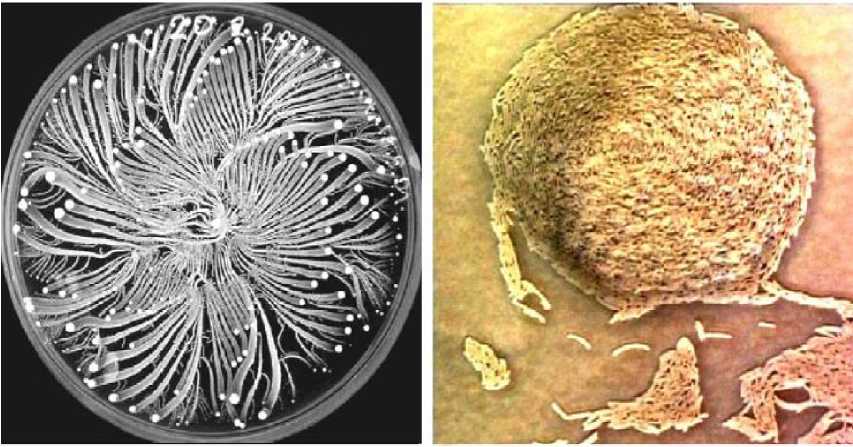
Figure 44. Hierarchical colony pattern generated by Paenibacillus vortex bacteria
Self-engineering capabilities of bacteria
Under natural growth conditions, bacteria can utilize intricate communication capabilities (e.g. quorumsensing, chemotactic signaling and plasmid exchange) to cooperatively form (self-organize) complex colonies with elevated adaptability – the colonial pattern is collectively engineered according to the encountered environmental conditions. Bacteria do not genetically store all the information required for creating all possible patterns. Instead, additional information is cooperatively generated as required for the colonial selforganization to proceed. A new picture is thus emerging, one in which adaptable self-engineering can be viewed as the bacteria solution to a challenging self-consistency mathematical problem at the forefront of optimization and control in nonlinear dynamics. So it is reasonable to conclude that collectively, bacteria can glean information from the environment and from other organisms and interpret the information in an existential «meaningful» way, i.e. by building an appropriate colony structure. It is perhaps even not so farfetched to imagine that the bacteria can develop common knowledge and learn from past experience.
Figs 45 and 46 show the main principles and robustness of self-engineering design systems.
Complex colonial forms (patterns) emerge through the communication-based singular interplay between individual bacteria (the micro-level) and the colony (the macro-level). Each bacterium is, by itself, a biotic autonomous system with its own internal cellular gel that possesses informatics capabilities (storage, processing and interpretation of information) ( Hellingwerf , 2005). These afford the cell certain freedom to select its response to biochemical messages it receives, including self-alteration and broadcasting messages to initiate alterations in other bacteria. Such self-plasticity and decision-making capabilities elevate the level of bacterial cooperation during colonial self-organization.
Forced mixing Engineered growth of air bubbles
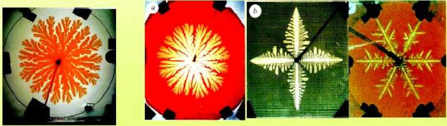
Figure 45. The idea of «Engineered Self-Organization» – «Forcing» the system to express its hidden «abili-ties»
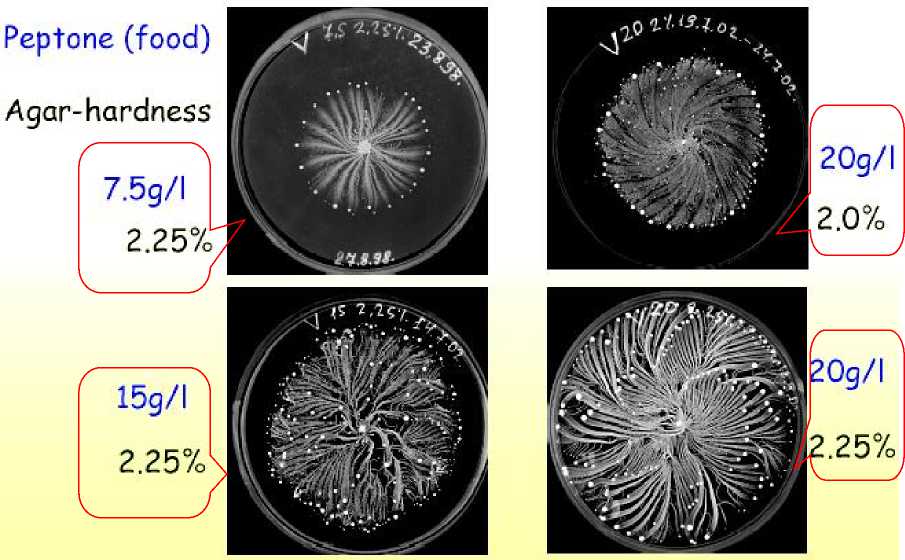
Figure 46. Robustness and specificity – The same P. vortex bacteria under different growth conditions
As the individuals in a growing colony begin to respond to the colony itself (i.e. information flow from the colony to the individual), these individuals response by regulating their movements, growth rates, various tasks they perform, the chemical signals they send to other bacteria and even their gene-network state (phenotypic state) according to the received signals.
Bacteria can perform most elementary cognitive function more efficiently as can be illustrated by their cooperative behavior (colonial or inter-cellular self-organization). As a member of a complex superorganism — the colony — each unit (bacteria) must possess the ability to sense and communicate with the other units comprising the collective and perform its task within a distribution of tasks. Bacterial communication thus entails collective sensing and cooperativity. The fundamental (primitive) elements of cognition in such systems include interpretation of (chemical) messages, distinction between internal and external information, and some self vs., non-self distinction (peers and cheaters).
Molecular biology is a subfield of biology that grew out of the fields of biochemistry, which is concerned with the chemical properties of living cells, and genetics, which is concerned with the evolutionary history of organisms and the relationships between them. The molecules of concern to molecular biology are those biochemical structures that are directly involved in encoding the information necessary for an organism to sustain its own life as well as to pass information to the next generation through the reproductive process. Main molecules are DNA, RNA and Protein.
DNA : Deoxyribonucleic acid. The double-stranded chemical instruction manual for everything a plant or animal does: grow, divide, even when and how to die. Very stable, has error detection and repair mechanisms; stays in the cell nucleus; can make good copies of itself. DNA is a polymer (a molecule) with two long complementary strands.
DNA bases – A: Adenine, T: Thymine, G: Guanine, C: Cytosine; DNA Base pairs: A ↔ T and G ↔ C . Human genome has approximately 3 ⋅ 10 9 bases and 15 ⋅ 10 3 genes.
RNA : Ribonucleic acid. Single-stranded where DNA is double-stranded, messenger RNA (mRNA) carries single pages of instructions out of the nucleus to places they're needed throughout the cell. No error detection or repair; makes flawed copies of itself. Evolves ten times faster than DNA. RNA is a polymer, a molecule related to DNA. Transfer RNA (tRNA) helps translate the mRNA message into chains of amino acids in the ribosomes. The expression of the genetic information in DNA is accomplished by transcribing a sequence of bases in DNA into a sequence of bases of RNA.
RNA bases – A: Adenine, U: Urile, G: Guanine, C: Cytosine. RNA Base pairs: A ↔ U and G ↔ C .
RNA differs from DNA in that it is single stranded and tends to fold back into itself forming hairpins. The DNA and RNA bases are also called nucleotides.
So these structures include DNA and RNA , each of which are strands of nucleotides ; these nucleotides cluster into groups of three to form amino acids , and these amino acids are the building blocks of proteins.
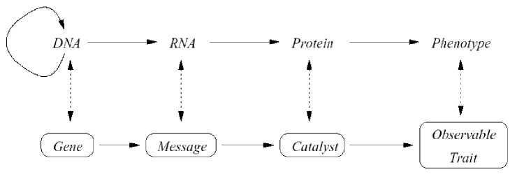
(a)
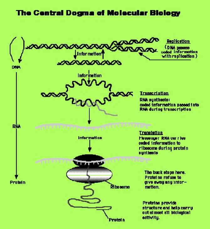
(b)
Figure 47. Structure of central dogma in molecular biology
What is known as the « central dogma » in molecular biology (see, Fig. 47) is the idea that the genome is the repository or template for all of the genetic information that is required both for organisms to perpetuate their own life and for them to pass this information on to the next generation through the reproductive process.
The central dogma initially stated that information in the organism flows from DNA to mRNA to protein in a unidirectional manner, but with the discovery of retroviruses and other organisms that transcribe genetic information from RNA to DNA and then back to mRNA to proteins, the unidirectionality rule has had to be relaxed.
The sequence hypothesis of molecular biology states that the sequences of nucleotides and amino acids determine the structure and function of the proteins that they code. The overarching goal of research in molecular biology since Watson and Crick first elucidated the sequence hypothesis in 1953 has been to discover just how these simple sequences of nucleotides are translated into proteins, and what impact the nucleotide sequence has on the 3-dimensional structure of proteins and function these proteins play within the organism.
The sequence of these nucleotides in turn determines what amino acids and proteins will be produced. If you consider the central dogma of molecular biology (at least for most prokaryotes and eukaryotes) that information moves from DNA to mRNA to protein, you can map this onto the model of a communication system we saw earlier. The source of the genetic message is the DNA strand.
Figs 48 and 49 are shown the structure of RNA.
Figure 48. Structure of RNA
DNA
ATGGCCTAAGCTCTGA
mRNA
UACCGGAUUCGAGACU
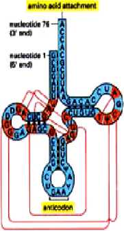
mRNA looks like DNA and is essentially a copy of a gene
“transfer" RNA (tRNA) is an adaptor used in protein synthesis
-
Figure 49. Two types of RNA
The message itself is the sequence of nucleotides in that strand. The channel is the RNA polymerase that recruits and attaches the proper nucleotides to the new mRNA strand, and the receiver is the mRNA strand.
The destination is the ribosome, which in turn initiates a process of translation from the sequence on the mRNA strand into proteins.
Errors or noise can be introduced as the RNA polymerase reads the DNA sequence and recruits the corresponding nucleotides (see, Fig. 50).
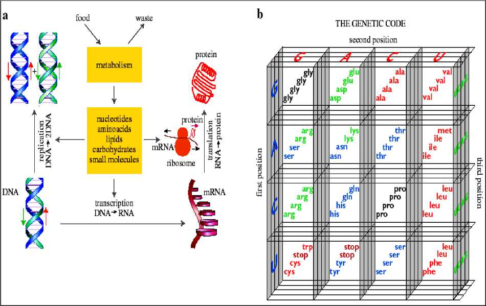
Figure 50. (a) Coupling between information processing and cellular metabolism; (b) The logical relationship between the nucleotide sequence of the nucleic acid and the amino acid sequence of the protein is the genetic code, which assigns an amino acid or a stop signal to each nucleotide triplet
In the translation step, mRNA is the source, the message is the transcribed nucleotide sequence, and the channel is the tRNA that directs the translation of nucleotide triplets (or codons) into amino acids (and is the place where noise in the form of translational errors can be introduced). The receiver is a polypeptide chain, and the destination of the completed protein can be any number of cellular structures that govern function in the cell.
The metabolism of the cell provides all the building blocks for the construction of the molecules present in the cell. Free energy, the driving force for these processes, comes from the conversion of food into waste products. Metabolism drives the elaboration of information in the cell, which can be expressed according to the central dogma of molecular biology.
The first step is transcription, which copies some of the DNA into RNA, which constitutes a sort of «working copy» of the genetic information. This RNA, called messenger RNA, is then translated into protein by a highly complex molecular mechanism involving the ribosome, a supra-molecular complex with many components.
Fig. 51 shows the entropy (in bits) for all pairs of bases of the set of E. coli sequences used to produce the entropy map, which demonstrates how the correlated paired bases in the four stems stand out [19]. This is endeavor proved successful, and the level of understanding is now such that we feel and can hint at a new approach to building complex man-made systems.
The human being central nervous system is composed of 10 11 - 10 12 neurons with about 10 16 synaptic connections.
Figure 51. Mutual entropy (information) between all bases (in bits), colored according to the color bar on the right, from 33 sequences of E. coli tRNA [19]
(The four stems are readily identified by their correlations as indicated)
A typical bacterial colony consists of 109 - 1012 bacteria. Both systems are not created by pre-design or according to a plan, but through a process of biotic self-organization. The elements (neurons or bacteria) do not store the information required to construct the system, but rather the information for creating the needed «tools» and the guiding principles. Additional information is cooperatively generated as the organization proceeds following external stimulation. The key principles that enable it are communication and selfplasticity of the components. The outcome is an adaptable complex system that can perform many tasks, learn and change itself accordingly.
Consequently, the idea of engineered self-organization is to let many collections of element selforganize in a pre-engineered environment they can exchange information with. The most efficient collections will be let to further self-improve via genetic algorithms of the components internal structure and capabilities (the analog of evolution of the potential for gene expression). The system itself should regulate the evolution of its components.
We can conclude with projections in regards to turning the conceptual idea, of engineered selforganization of communicating elements with self-plasticity, into an operational approach that will enable the creation systems too complex for design, yet with desired pre-specified capabilities.
Role of quantum correlations and information transport in self-organization models
For QA design of self-organization based on QFI-model we will use examples of novel informationtransport and self-organization processing mechanisms in nanometer-scale structures based on different types of quantum correlations. The local modulation and detection of a quantum state can be used for information transport at the nanometer length-scale, an effect called a « quantum mirage » [50 – 52].
Unlike conventional electronic information transport using wires, the quantum mirage can be used to pass multiple channels of information through the same volume of a solid. Nanometer structures offer the possibility of fundamentally different ways to transport and process information, and the ‘clunk’ in computational structures, so far as physical limitations are concerned, is not encountered, at least down to nanometer dimensions.
A new class of nanometer-scale structures called ‘molecule cascades’ was discussed [50], and show how they may be used to implement a general-purpose binary-logic computer in which all of the circuitry is at the nanometer- length-scale. Bottom-up approach is one of the main focus research areas of nanoscience where various atomic structures will be constructed on an atom-by-atom basis. Manipulation with a scanning tunneling microscope (STM) tip allows engineering of man-designed structures using single at-oms/molecules or investigating the physical/chemical properties of materials at an atomic level. Positioning of single atoms with subatomic level precision on a surface requires an extremely fine control over the tipatom-surface junction. The detailed knowledge of how an atom moves across a surface is valuable for both fundamental understanding and further progress of nanoscience.
-
A . Definition of Quantum Mirage . According to the definition «Quantum Mirage» is as following: A nanoscale property that may allow information to be transferred through use of the wave property of electrons. Thus, quantum computers might not require wires as we know them.
Quantum Wire : Another form of quantum dot, but unlike the single-dimension «dot», a quantum wire is confined only in two dimensions – that is it has «length», and allows the electrons to propagate in a «parti-cle-like» fashion. Constructed typically on a semiconductor base, and (among other things) used to produce very intense laser beams, switchable up to multi-gigahertz per second.
Fig. 52 shows the effect of quantum mirage in Cu(111) quantum dot.
-
B . Surface states and quantum corrals . The Cu(111) surface has surface-state electrons that form a nearly ideal two dimensional non-interacting electron gas. These surface-state electrons are scattered by step edges and defects creating standing waves in the local density of states (LDOS) that are readily imaged with the scanning tunneling microscope (STM) (see Crommie et al . 1993 a ). Crommie et al (1993 b ) showed how these electrons could be confined in-plane to structures called «quantum corrals».
Remark. Quantum corrals are built by positioning atoms, typically transition metal atoms, along a closed line on the clean surfaces of noble metals. In recent experiments Manoharan et. al have built elliptical corrals with Co atoms on the (111) surface of Cu. The Cu (111) surface (see, Fig. 52) has a band of surface states, orthogonal to the bulk states, which can be represented as a two dimensional electron gas confined at the surface. The Fermi level is placed at 450 meV above the bottom of the surface state band. The atoms forming the corral act as scattering centers which tend to confine surface electrons inside the corral. If the corral fence where an impenetrable wall electrons inside the corral would be perfectly confined and the energy spectrum would consist of a set of delta functions at the energies of the bound states. The characteristic energy separation between these states decreases as the size of the corral increases. In real systems, there is some leaking of the wave function: electrons can tunnel through the fence and the bound states acquire a finite life time. The energy spectrum inside the corral (the local density of states) then consists of resonances, the width of which increases with increasing energy.
Figure 52. The example concerns a novel method for information transport
[The quantum-mirage effect – The Cu(111) surface (Manoharan et. al, 2000, [52])]
-
C . Role of correlation types in quantum corral self-organization . The fabrication of solid state quantum computing devices involves both the ability to manipulate mater at the nanoscale and to design structures that interact according to prescribed quantum computing Hamiltonians. Tuning and controlling quantum interactions are basic problems faced by the quantum computing community. This requires engineering the structure of electronic wave functions in different environments and conditions. The manipulation of individual atoms with STM has made possible the construction of arbitrary quantum structures on top of surfaces.
Quantum corrals are a collection of atoms arranged in a controlled manner on top of a metallic surface. These novel structures generate quantum confinement of the surface conduction electron wave functions leading to striking phenomena such as resonant electronic states and the formation of quantum mirages. Generally speaking, quantum mirages are the projection of a perturbation on a point into another distant point of the surface. The magnetic interaction between magnetic impurities can be strongly enhanced due to the electronic confinement produced by quantum corrals.
Example : Design of a quantum corral to generate chosen couplings between three spins . In general, to lowest order, the magnetic behavior of a collection of impurities at coordinates { R } is given by the following target Hamiltonian [51]:
H .„=2-3, v,=2 JJjC (Ri. Rj). (3) i. j i. j where the summation is done over all impurity pairs. The exchange parameters can be written as J.. = J.J.C(R. Rj) with the corresponding correlation function C (R. Rj).
Case 1 : A single mirage . To test of method in this simple case, the simulated annealing algorithm was instructed to maximize the quantity C ( Rx,R 2) , i.e. to project a perturbation from Rx to R 2 as efficiently as possible. The cost function was chosen to be simply Ex = — C ( Rx,R2 ) . The reflection symmetry at the x -axis was imposed on the corral impurities to simplify the problem. The distance between the spins at R and R was fixed to 140 A o to resemble the experimental conditions. Once the optimization procedure is completed, the correlation function is plotted in [51].
Fig. 53 shows the response function and the quantum corral resulting form optimization process. For the results case of Fig. 53 we have: H
—J • 5 1 • s 2 .
Figure 54. Case 2
Figure 53. Case 1
Fig. 53 also shows that the minimum found presents some resemblances to the ellipse but new unexpected features also appear. First of all, the atoms of the corral tend to accumulate around the location of the perturbation and also around the location of the desired mirage. Atoms on the long sides have less importance and are placed in a less dense arrangement.
This contrasts with the evenly spaced atoms of the early experimental setups. A second shell of impurities appears to be more efficient than a single shell to confine the electron gas and produces better mirages.
For comparison the family of con-focal ellipses have studied that can be formed with the same number of equidistant impurities (being the perturbation at one focus and the mirage at the other). The best mirage was finding that formed by the family as a factor 3 smaller than the one obtained with the structure shown in Fig. 53.
Case 2 : A complex mirage . Suppose now that we want to build a quantum corral such that generates a target magnetic Hamiltonian of three impurities:
Htarget = -* si * s2 - J * si * S3 , i.e. only a selected set of pairs of the three spins are coupled. We arbitrarily choose the coordinates of the spins R , R and R to be in the vertexes of an equilateral triangle of side d = 121 Ao .
Note the following: (i) the last equation is a particular case of Eq. (3) where J 23 = 0 and JXT = <У23 = J ; and (ii) the target Hamiltonian has a different symmetry than the desired positions of the magnetic spins.
That is, we require the magnetic couplings on two sides of the triangle but not on the third. The resulting corral is shown in Figs 53 and 54; the original requirements are efficiently achieved in [51].
In Fig. 54 the optimum configuration found for the impurity atoms has dense focusing structures near the source of the perturbation and near the mirages. Amazingly, some atoms are automatically located in the middle of the corral to split the standing waves towards the «targets» at R and R .
-75 -50 -25 0 25 50 75 100
Figure 55. Case 3
-75 -50 -25 0 25 50 75 100
Figure 56. Case 4
Fig. 55 (case 3) shows the effect of a magnetic impurity at R which produces a large response at R but not at R [in contrast with the case of an impurity located at R (compare with Fig. 54)]. The corral is the same in Figs 53 and 54; the difference is the position of the magnetic perturbation.
Comparison of Figs 54 and 55 shows that the interaction will induce couplings as initially designed. The resulting magnetization shows that s and s are not directly coupled . At the same time the interactions between s and s , and between s and s are enhanced. The positions of the spins and the Hamiltonian chosen are arbitrary.
The resulting design for four spins with a target Hamiltonian:
H target = - J ⋅ s 1 ⋅ s 3 - J ⋅ s 2 ⋅ s 4 (4)
where the positions of the spins form a square.
The results of minimizing are shown in Fig. 56 (case 4). Fig. 56 shows the spin density generated by a perturbation at R . The spin density when the magnetic perturbation is at R gives another position of corral. Therefore, the spin Hamiltonian formed by this structure has two pairs of spins interacting independently. Each pair of spins does not couple with the other pair, even though the interaction is mediated by an electron gas that is shared by both pairs. Thus the designed structure of corral is dependent from type of quantum correlation [11, 51, 52].
-
D . Role of information-transport in quantum corral self-organization . Let us now to discuss two examples of novel information-transport and processing mechanisms in nanometer-scale structures. The local modulation and detection of a quantum state can be used for information transport at the nanometer lengthscale, an effect we call a « quantum mirage ». Unlike conventional electronic information transport using wires, the quantum mirage can be used to pass multiple channels of information through the same volume of a solid. A new class of nanometer-scale structures called ‘molecule cascades’ is discussed [11, 25], and show how they may be used to implement a general-purpose binary-logic computer in which all of the circuitry is at the nanometer length-scale. The power dissipated in mirage-based information transport is independent of the distance over which the information is transported. The detection of the mirage necessarily requires creation of either particle-like or hole-like excitations in the quantum system and is thus dissipative.
Example : Multi-channel information transport . One of the most intriguing capabilities of mirage-based information transport comes from its wave-coherent nature. In the non-interacting limit, the electrons of a system can be considered as independent and the principle of superposition holds true. This suggests that, as with classical waves, we should be able to transmit multiple channels of information through the same volume of space by selectively modulating spatially overlapping quantum states.
Fig. 57 shows how two channels of information could be transported in a crossed-ellipse-shaped quantum corral specifically designed for this purpose [50].
The mirages shown in ( h ) demonstrate the ability to pass two channels of information through the same volume of space using the quantum-mirage effect [50].
While it is true that electrons always interact with each other and a system of electrons must be properly described by a many-body wave function, Fig. 57 demonstrates that there are regimes in which the singleparticle non-interacting approximation is useful and the isolation between channels is more than adequate for the transmission of binary information.
The successful application of multi-channel information «cross-troughs», such as that shown in Fig. 57, has the potential to significantly reduce the number of wiring layers in a chip.
We will discuss a novel mechanism of nanostructure growth based on quantum confinement of surfacestate electrons.
Ab initio calculations and the kinetic Monte Carlo simulations reveal the phenomenon of confinement-induced adatom self-organization in quantum corrals.
The studies indicate that new atomic scale nanostructures can be engineered exploiting the quantum confinement of surface electrons.
Figure 57. Multi-channel information transport with the quantum mirage
(a), (c), (e), (g) STM topographs of crossed-ellipse structure. (a) No atoms at foci of ellipses; (c) atom at left focus; (e) atom at top focus; and (g) atoms at left and top foci. (b), (d), (f), (h) dI/dV difference images corresponding to the topographs (a), (c), (e) and (g), respectively. (b) No mirage; (d) mirage at right focus; (f) mirage at bottom focus; (h) mirages at both right and bottom foci
-
E . Adatom self-organization induced by quantum confinement of surface electrons . As above mentioned noble metal surfaces featuring a surface state are especially appealing substrates to study quantum confinement. It is known that surface-state electrons on (111) noble metal surfaces form a two-dimensional (2D) nearly free electron gas. Particularly fascinating phenomena occur if the surface electrons are confined to closed structures (corrals). The direct observation of standing-wave patterns in the Fe corral on Cu(111) is one of the most spectacular examples demonstrating quantum effects at the atomic scale. The quantum confinement of surface electrons inside corrals can lead to a mirage effect, i.e., the projection of the electronic structure of adatoms to a remote location. Quantum corrals can be used to tailor the spin polarization of surface electrons and magnetic interactions between adatoms.
We will concentrate on self-organization properties on Co adatoms on Cu(111) and Ce adatoms on Ag(111) confined to quantum corrals, and demonstrate a novel mechanism of quantum growth on metal surfaces. The self-organization of adatoms inside corrals has been revealed. One of the most important aspects in nano-science is the formation of artificial nanostructures. Ordered structures of atoms and molecules can be generated either by the manipulation of single atoms or molecules by means of the tip of a scanning tunneling microscope or by using self-assembly processes of particles.
Fig. 58 shows the self-organization process in a man-made atomic ring and the interference pattern of electrons «confined» in this structure.
Surface-state electrons are confined within the corral by strong scattering at the corral walls. The quantum interference between electronic waves traveling towards to the corral walls and the backscattered ones leads to the standing-wave patterns. In other words, strong oscillations in the LDOS manifest the confined surface states. The interaction of the confined surface electrons with adatoms leads to an interesting effect. The energy of the Co adatom placed inside the corral is calculated. For large distances between the adatom and the corral walls the interaction energies are calculated in the framework of the frozen potential approximation using single-particle energies instead of total energies. The energy exhibits an oscillatory behavior and can be attractive or repulsive. For the adatom it appears to be energetically favorable to rest in regions of high LDOS. These results clearly demonstrate the impact of the quantum confinement of surface electrons on energetics of adatoms.
The quantum confinement of surface electrons and the surface-state mediated long-range interactions with spatial quantum correlation are shown to determine the growth process in quantum corrals based on self-organization possibilities.
Structure evolution process of quantum dot design
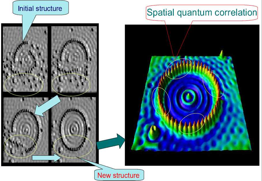
Figure 58. Self-organization in quantum dot
Qualitative description of quantum effects in self-organization processes
Let us consider the common parts of models of self-organization processes of natural evolution processes according to abovementioned Items 1 and 2 of our results in this paper.
As example we are consider pedestrian walkway flow in different crowd types.
Fig. 59 shows the different types of pedestrian walkway flows.
What the common operators of flow description can we observe from Fig. 59?
For a crowd in Fig. 59a (Box 1 ) we can to see that self-organization process of pedestrian flow based on superposition of people pairs that illustrated in Fig. 60.
In analogy Fig. 61 is demonstrated the communication process between pedestrian pairs with the quantum entanglement for a crowd in Fig. 59a (Box 2).
The role of quantum interference is demonstrated in Fig. 62 in the case of a crowd in Fig. 59a (Box 3).
Fig. 59b is demonstrated the role of quantum temporal correlation in the self-organization of pedestrian flow in crowd. Fig. 58 shows the quantum spatial correlation in quantum dot structure of evolution design.
Thus the self-organization process can be considered as the classical process on macro levels with quantum effects in hidden (micro) levels.
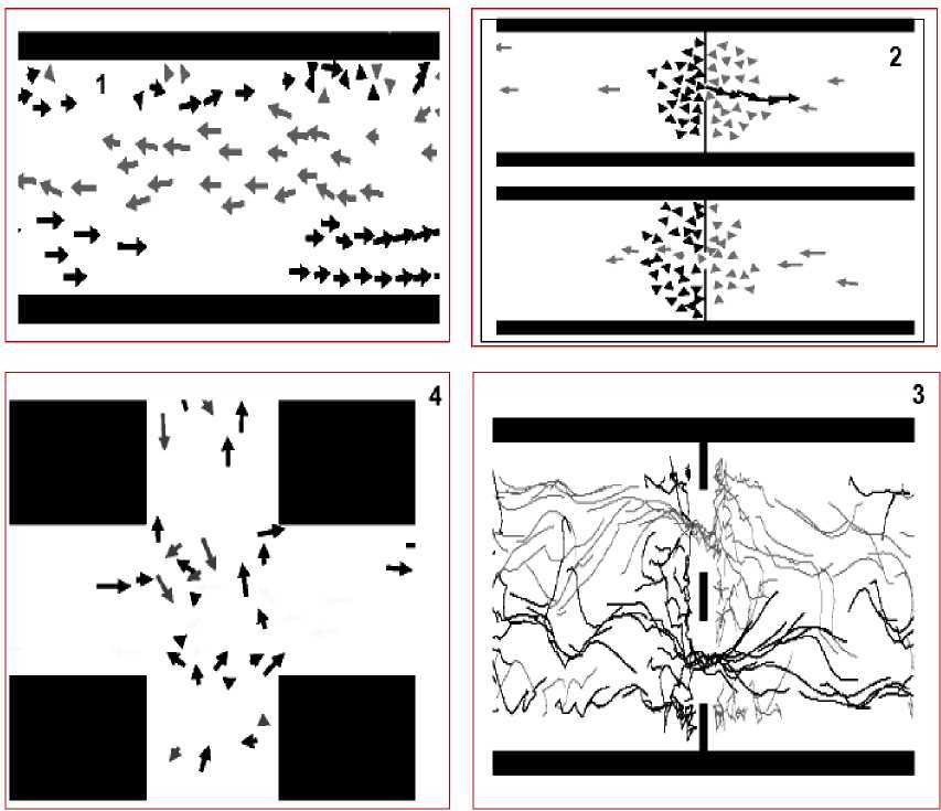
(a)
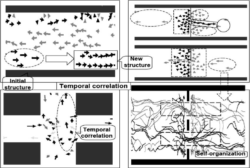
(b)
-
Figure 59. Structure of pedestrian walkway in crowds
-
(a) – types of pedestrian walkways; (b) – types of quantum correlation in self-organization
1. Classical case
1.Quantum superposition of particles
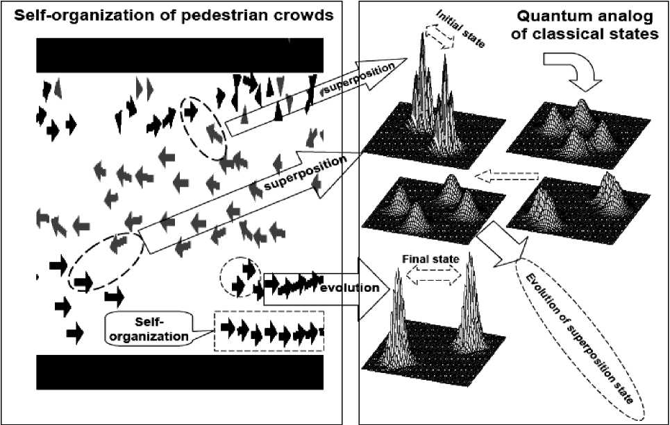
Figure 60. Creation of superposition in pedestrian crowd flow
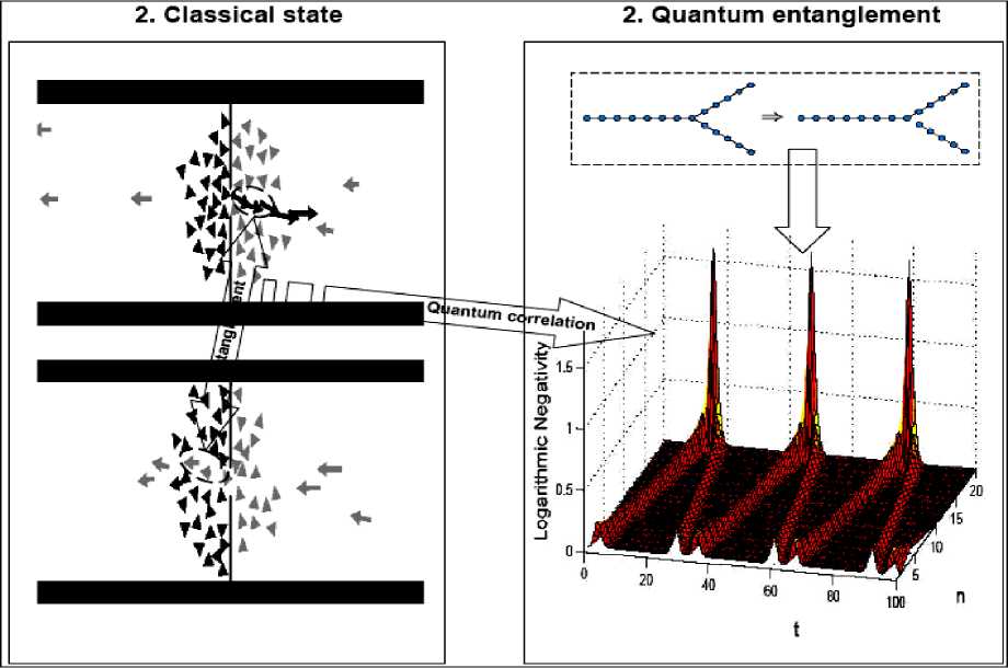
Figure 61. Communications between pedestrian pairs in a crowd with quantum entanglement
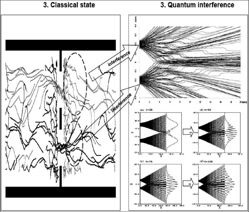
Figure 62. Interference of pedestrian flow in crowd
Remark . The structure of quantum fuzzy inference (QFI) model that realize the self-organization process is a new quantum algorithm. QFI is one of possible realization of quantum control algorithm of the selforganization processes that includes all of these features: (i) superposition; (ii) selection of quantum correlation types; (iii) information transport and quantum oracle (dynamic evolution); and (iv) interference. QFI model is introduced based on thermodynamics and information-theoretic measures of agent interactions in communication space between macro- and micro-levels (the entanglement-assisted correlations in an active system represented by a collection of intelligent agents). From computer science viewpoint, QA of QFI model plays the role of the information-algorithmic and SW-platform support for design of self-organization process. Physically, QFI supports optimal thermodynamic trade-off between stability, controllability and robustness in self-organization process. The dominant role of self-organization in robust knowledge base (KB) design of intelligent fuzzy controllers (FC) for unpredicted control situations is discussed.
General Structure of QA of Self-Organization Processes
Fig. 63 shows the general structure of QA for logical design of bio-inspired self-organization process (see, Fig. 7) that includes these common parts.
Algorithmic Level
Natural Decoding o Solution & A nswer
Final
New Self-Organized Robust Structure Decision
Operator
(self-organization) Operator (Self-assembly)
( Evolution Dynamic )( Problem-Oriented Correlation )
Vector (Templating of structure) components
Initial
Random (Classical/Quantum) Search
Classical, Quantum, or Mixed Types
Genetic Inspired Initial Structure
Action of operat
operator
Action of
CL
C O)
Algorithmic description
Search
States with idden Informatio
Choice
Coding of Problem
lgorithm des ign of Self-Organization with Problem-Oriented Operators
Figure 63. Quantum Algorithm of logical design of bio-inspired self-organization process
Quantum swarm algorithm
It is a QA design of self-organization with problem-oriented quantum operators:
-
- First step of algorithm, initial states are vector-state that describes component’s templating of future designed structure. From bio-inspired structure point of view it is genetic inspired initial structure of evolution process; from computer science stand viewpoint it is coding of problem searching solution. It is well-known in computer science that vector and matrix can be presented using quantum state: The quantum representation of vector and matrix may be the base of quantum data structure (for compression presentation of massive classical data [21] in templating);
-
- On second step of algorithm a self-assembly process is used (from bio-inspired structure point of view); from computer science stand viewpoint it is a decision-making process on choice of problem-oriented correlation. An action of correlation operator on initial state in templating prepare a structured assemble of components with hidden possible solutions of design structure;
-
- Evolution dynamic realize a self-organization process of new structure design on the third step. Algorithmic description of self-organization process is a random quantum search process of hidden solution in self-assembly structure and acts as corresponding operator on self-assembly structure;
-
- Natural decoding of searching solution is given the answer about final state of a new self-organized structure.
The described algorithm is in general a quantum control design algorithm that includes all operation from general structure of QA.
Remark. In this section we briefly consider analogy with structure of a QA [22, 23]. In the following section, further concepts of quantum computing will be introduced that will be necessary to apply the de- scribed methodology. General structure of QA consists from three quantum as superposition, entanglement (quantum correlation) and interference. Classical measurement gives the final result of quantum computation. Superposition operation is realized by Hadamard transform, entanglement is realized by CNOT-operation or by quantum oracle, and interference is realized by QFT-operator. Main goal of QA applications is the study and search of qualitative properties of functions as the solution of problem. Initial states are coding of function property. Superposition describes the generalized searching space; a quantum oracle finds the searching solution; with interference operator and classical measurement the searching solution is extracted. The method of collective behavior (swarm method) is the simplest and most evident way for the algorithmization of quantum models. The passage from the single particle to the swarm of its samples seems to be the easiest way to overcome contra intuitiveness featured to quantum theory. With some additional suppositions a swarm method gives the algorithm of simulation of the dynamics with linear complexity of the number of particles. These additional suppositions lay in the framework of the basic idea of algorithmic approach the limitation of the memory and time for the simulation [1, 24].
Fig. 64 shows the general structure of QA [11].
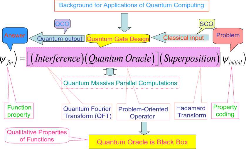
-
Figure 64. General structure of quantum algorithm
The superposition is that we should treat as realizable only states of the system S = S n S 2, s sup S 2 = 0 of the form [24]
I ^ s )= E x j Vti 0 I j , (5)
where | ^ 1 J, | V !),••• and | ^ 12), I V 2 ) are orthonormal basis in space of states of subsystems S and S2 correspondingly, and each of these basic states has the same form, with some depth of nesting. Factually, this is one particle states, where the entanglement is distributed among the particles sequentially nested in each other.
The quantum swarm model of self-organization was described in [1].
Remark. Based upon quantum entanglement, several paradigms of self-organization (such as inverse diffusion, transmissions of conditional information, decentralized coordination, cooperative computing, competitive games, and topological evolution in active systems) can be introduced and discussed. This result was motivated by recent discovery and experimental verification of the most fundamental and still mysterious phenomenon in quantum mechanics: quantum entanglement. Formally, quantum entanglement as well as associated with it quantum non-locality follows from the Schrödinger equation; however, its physical meaning is still under extensive discussions. The most attractive aspect of quantum entanglement, in terms of a new quantum technology, is associated with instantaneous transmission of messages on remote distances. However, practical applications of this effect are restricted by the postulate adopted by many authors that these messages cannot deliver any intentional information. That is why all the entanglement-based communication algorithms must include a classical channel. The main challenge of this study is to evaluate the degree of usefulness of entanglement-based communication technology without any classical channels. The first attempt of this kind has been demonstrated how a randomly chosen message can deliver non-intentional, but useful, information under special conditions which include a preliminary agreement between the sender and the receiver. This effort can be to extend by applying the entanglement-based correlations to an active system represented by a collection of intelligent agents. The problem of behavior of intelligent agents correlated by identical random messages in a decentralized way has its own significance: it simulates evolutionary behavior of biological and social systems correlated only via simultaneous sensoring sequences of unexpected events.
As shown in this report that under the condition that the agents have certain preliminary knowledge about each other, the whole system can exhibit emergent phenomena such as a new robust KB of intelligent control system for unpredicted control situations. It also can perform transmission of conditional information, decentralized coordination, cooperative computing, competitive games, topological selforganization, and inverse diffusion [1, 11, 25].
Quantum control algorithm of self-organization processes
Let us consider the peculiarities of common parts in self-organization models (presented in Fig. 7) [11]:
-
(i) Models of self-organizations on macro-level are used the information from micro-level that support thermodynamic relations (second law of thermodynamics: increasing and decreasing of entropy on micro-and macro-levels, correspondingly) of dynamic evolution;
-
(ii) Self-organization processes are used transport of the information on/to macro- and from microlevels in different hidden forms;
-
(iii) Final states of self-organized structure have minimum of entropy production;
-
(iv) Types of correlation in natural self-organization processes are don’t planning before the evolution (Nature given the type of corresponding correlation through genetic coding of templates in self-assembly);
Coordination control for design of self-organization structure is used;
Random searching process for self-organization structure design is applied;
-
(vii) Natural models are biologically inspired evolution dynamic models and are used current classical information for decision-making (but don’t have toolkit for extraction and exchanging of hidden quantum information from dynamic behavior of control object).
In man-made self-organization types of correlations and control of self-organization are developed before the design of the searching structure.
Thus the future design algorithm of self-organization must include these common peculiarities of bioinspired and man-made processes: quantum hidden correlations and information transport .
Fig. 65 shows the structure of a new quantum control algorithm of self-organization that includes the above mentioned properties.
Remark . The developed quantum control algorithm includes three possibilities: (i) from the simplest living organism composition in response to external stimuli of bacterial and neuronal self-organization; and (ii) according to correlation information stored in the DNA; (iii) from quantum hidden correlations and information transport used in quantum dots.
Quantum control algorithm of self-organization design in intelligent control systems based on QFI-model is described in [1, 11]. In particular case, QFI model is the background of robust KB design information technology.
Main goal of quantum control algorithm of self-organization in Fig. 65 is the support of optimal thermodynamic trade-off between stability , controllability and robustness of control object behavior using robust self-organized KB of intelligent control system.
Robust
KB
Final State)
Self -Organized Robust Structure
Goal : Support of Optimal Thermodynamic Trade-off between Stability , Controllability and Robustness
Level 3
Feedforward Design
o>
I Quantum Control Algorithm of Self-Organization
.2 I о
ro
Ф
Ф
State with Hidden Quantum
Information
= ( Evolution Control Dynamic )( Problem - Oriented Correlation ) | Initial State)
Random (Classical/Quantum) Search | ) > Classical, Quantum, or Mixed Types | ) )_ Genetic Inspired State
Level 2
Natural Bio-Inspired Self-Organization
Environment Case-Study
/ £
Level 1
/ CO/

Quantum Self-rganizatio
Action
SelfAssembly
Computational Intelligence
Quantum Fuzzy Inference
Apply
Action Templating
Algorithmic Toolkit
Decision Making and Properties Choice
Soft
Apply Computing
Optimizer
-
Figure 65. Structure of quantum control algorithm of self-organization
Related works. In many publications the models of self-organizations are described [2-10, 18, 53-57] etc. In mentioned publications quantum control algorithms of self-organization is not introduced. Our paper is a generalization of abovementioned publications. Present paper has extended analysis of self-organization models on five levels that differ in principle from abovementioned publications. The result of this work is the description in detail the developed quantum control algorithm of self-organization that includes a new quantum operator types for design quantum control of self-organization processes.
Conclusions
As formulated analysis of self-organization models described in this paper gives us the following results:
-
1 . Natural evolution processes are based on the following steps [2 – 7]:
-
(i) templating ; (iii) self-assembling ; and (iii) self-organization .
-
2 . Models of self-organization are included natural quantum effects and based on the following information-thermodynamic concepts:
-
(i) macro- and micro-level interactions with information exchange (in ABM micro-level is the communication space where the inter-agent messages are exchanged and is explained by decreased entropy on a macro-level and increased entropy on a micro-level);
-
(ii) communication and information transport on macro- and micro-levels («quantum mirage» in quantum corrals);
-
(iii) different types of quantum spin correlation that design different structure in self-organization (as example, quantum dot);
-
(iv) coordination control (swam-bot and snake-bot).
We choice for analysis of common futures as Benchmarks the following examples [2–19]:
-
(1) Pedestrian behavior and self-organization;
-
(2) «Phantom panics» and self-organization;
-
(3) Self-organization of traffic flow models;
-
(4) Swarm self-organization and swarm intelligence (SI):
-
4.1 . Applications of SI and ant colony self-organization;
-
4.2 . Agent-Based Models (ABM);
-
4.3 . Quantum cooperation of two insects;
-
4.4 . Engineered self-organization of a bacteria colony;
-
-
(5) Self-organization in nano-scale structures: Quantum corrals .
As can we to see different models of self-organization processes are described from physical, information, and algorithmic (quantum computing) point of view. Role of quantum correlation types and information transport in self-organization of structure type design was discussed. The physical interpretation of self-organization control process on quantum level is introduced and based on the information-thermodynamic model of the exchange and extraction of quantum (hidden) value information from/between classical particle’s trajectories in particle swarm. New types of quantum correlations (as behavior control coordinator) and information transport (value information) between particle swarm trajectories are introduced.
Q: Why self-organization control algorithm is quantum?
A : (i) In quantum computing theory every QA in general form includes the following unitary quantum operators: (i) superposition; (ii) entanglement (quantum oracle); (iii) interference. Measurement is the fourth classical operator. [It is irreversible operator and is used for measurement of computation results].
-
(ii) The developed algorithm of self-organization includes these operators.
-
(iii) With superposition is realized templating operation, and based on macro- and micro-level interactions with information exchange of active agents.
-
(iv) Selection of quantum correlation type is dependent from the properties of concrete nonlinear systems and organize self-assembling using power source of communication and information transport on micro-level.
-
(v) Quantum oracle calculates intelligent quantum state that includes the most important (value) information transport for coordination control.
-
(vi) Interference is used for extraction the results of coordination control and design in on-line robust self-organization structure.
References Role of information-thermodynamic trade-off models of control qualitative in quantum control algorithm of self-organization design
- Ulyanov S.V., Litvintseva L.V., Ulyanov S.S. Quantum swarm model of self-organization process based on quantum fuzzy inference and robust wise control design // Proc. 7th International Conference on Application of Fuzzy Systems and Soft Computing (ICAFS'2006). - Siegen, Germany, September 13-14, 2006. - Pp. 10-19.
- Camazine S., Deneubourg J.-L., Franks N.R., Sneyd J., Theraulaz G., Bonabeau E. Self-organization in biological systems. - Princeton University Press, 2003.
- Hemelrijk C.K. (Ed.) Self-organisation and evolution of social systems. - UK: Cambridge University Press, 2005.
- Helbing D. Traffic and related self-driven many-particle systems // Reviews of Modern Physics. - 2001. - Vol. 73. - № 4. - Pp.1067-1141.
- EDN: LZXAEV
- Czap H., Unland R., Branki C., Tianfield H. Self-organization and autonomic informatics. - Springer Verlag (Frontiers in Artificial Intelligence and Applications), 2005. - Vol. 135.
