Rough Neuron network for Fault Diagnosis

Published Online March 2011 in MECS

Intelligent fault diagnosis is an important developing direction of diagnostic technique. The traditional fault diagnosis method is based on the mathematical model of the system, mathematical model is dependent on the diagnosis system structure in [1], but many faults can cause changes in the structure of the system. Neural network technology has self-learning, nonlinear pattern recognition, associative memory and presumed ability, good fault tolerance and expansibility, so fault diagnosis is widely used in [2-4]. There are also many scholars improved neural network, for example, reference [5] optimized BP neural network with L-M method, there are many virtues such as fast convergence and hard into the local minimum values for the network. self-learning ability of BP neural network and interpreting ability of expert system is combined in [6], reliability and accuracy of system are increased.

But when the input information dimension becomes large, the above training time of neural network is too long. Rough Sets Theory was proposed in 1982 by Pawlak in paper [7] ,it is a new mathematical tool to deal

Footnotes: 8-point Times New Roman font;

Manuscript received January 1, 2008; revised June 1, 2008; accepted

July 1, 2008.

Copyright credit, project number, corresponding author, etc.

with vagueness and uncertainty. In reference [8-10], it has been applied in many areas such as pattern recognition, data mining and fault diagnosis. Its reduction operation can remove redundant attributes and redundancy samples, compression information space dimension, simplify the knowledge system, realize The pretreatment of information system. Literature[11,12] used Rough Sets Theory for pretreatment of input data of neural network, extracting key ingredients as input of network, although simplified structure of the neural networks, the operation mechanism of neural network was not improved.

This paper proposes a new neural network base on rough neuron, rough neuron network model bycombining rough set theory with neuron concepts, which has broad meaning in real world. Rough neuron network can solve input vector with multiple-valued effectively. A new kind of Rough neuron network is proposed and applied in fault diagnosis.

П . Preliminaries and notations

• A.    Basic concepts of Rough Set

Definition 1 Let an information system is a 4-tuple S = ( U , A, V , f ) , where U is an objects collection (Domain); A = C U D is an attribute set, subset C is called condition attribute and D is called decision attribute; A is an attribute set; V is a set of attributes,

V = U Va ; f : U x A ^ V is an information function, a e A which designates each object a e A , x e U , f (x,a) e Va. The information system that provided with condition attribute and decision attribute is called decision table.

Definition 2 Let an information system is a 4-tuple S = ( U , A , V , f )      , defined the set

R ( X ) = { x e U |[ x ] _R с X } as X ’s lower approximation set, and R ( X ) = { x e U |[ x ] _R I X ^ ф} as X ’s upper approximation set.

Definition 3 Let an information system is a 4-tuple

S = (U, A, V, f), defined the set U {x e U |[x]c с X} xeU / D as positive region of set D in set C , marks as POSIND(C) (IND(D)) or POSC(D) .

Definition 4 Let an information system is a 4-tuple S = (U , A, V , f ) , A = C U D and the dependability between D and C is defined: k = y c ( D ) = POS c ( D )|/ ^ |. For the attribute of c e C , if y_c ( D ) = y_c - c ( D ), then attribute c is redundant attribute which is relative to decision-making attribute D . Or it is indispensable attribute. Under the importance of C relative to D , attribute c is defined: SSGF ( c , C , D ) = y _c ( D ) - y_C - c ( D ) . If any attribute is indispensable in C relative to D , then C and D are independent.

Definition 5 Let an information system is a 4-tuple S = ( U , A , V , f ) , A = C U D and P e C . If P and D are independent, and y_c ( D ) = у_p ( D ) , then P is called C ’s relative reduction of D , and marks as RED ( C ) .

• B.    Rough Neuron

A rough neuron in reference [13] can be regarded as consist of two or d inary neurons, one of them is called the upper boundary r , the other is called the lower boundary r , as shown in figure 1.

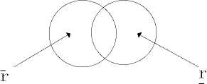
Figure.1 Rough neuron.

The input of a conventional, lower, or upper neuron is calculated using the weighted sum as:

inputs = ^ to ji x output j                   (1)

j where i and j are either the conventional neurons or upper/lower neurons of a rough neuron. The outputs of a rough neuron r is calculated using a transfer function as:

output-r = max( f (input-), f (inputr))(2)

output r = min( f (input-r), f (input r))(3)

The output of a conventional neuron i is simply calculated as:

outputt = f (inputi)(4)

The connection between the upper boundary and the lower boundary represents information exchange, there are three kinds of connection between a rough neuron and another rough neuron, as shown in figure 2, Where figure 2-a shows fully connected between rough neuron r and s ; figure 2-b shows rough neuron r incents rough neuron s ; figure 2-c shows rough neuron r inhibits rough neuron s .

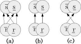
Figure 2. Rough neurons connection graph.

When the connection between neurons is existent, input formula of the upper boundary or the lower boundary neurons can be expressed as I j = ^ rn ij x O i , neuron i and neuron j may be classic neuron, also can be the upper boundary or the lower boundary of rough neuron. Output formula of rough neuron can be expressed as O r = max{ f ( P ), f ( I_r )} , O_L = min{ f ( L ), f ( I_r )} , function f using Sigmoid function.

• C.    Rough Neuron BP Neural Network

Rough neural network is the neural network which enabled the input value that considered an accidental error by having a revolving underwriting facility neuron into input with a rough set theory. It gets possible to handle uncertain data than a rough neuron. I can think about a rough neuron in rough neural network like a pair of a neuron. Therefore I can gain the favor by a rough set theory as a rough neuron and define two normal neuron as revolving underwriting facility neuron of one and take a lower limit of input as the other with an upper limit of input including an accidental error for one input as input of revolving underwriting facility neuron.

According to the traditional BP neural network, input value of each neuron is a precise value, but it may be two values or multiple values in some practical problems. Rough BP neural network can solve these problems. It is similar with traditional BP network, consists of threelayered feed forward network, namely: input layer, hidden layer and output layer, using fully connected between each layer. As shown in figure 3, input layer consists of rough neurons, each rough neuron is consist of two ordinary neurons, hidden layer or output layer is consist of ordinary neuron.

Hidden layer

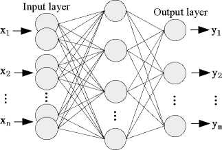
Figure 3. Rough neuron BP neural network.

Ш . Attribute discretization based pso

Rough Sets Theory only deal with discretized data, so the continuous attribute should be discretized at first, then reduction by using Rough Sets Theory. Meanwhile, it is very important to increase running speed of learning algorithm in next step, reduce actual space requirements and time consumption of algorithm, improve clustering ability.

• A.    Definition of Generalized Discretization

The main point of the existing discretization definition [14] is that condition attribute space is split using selected cuts. The existing discretization methods [14-17] always try to find the best cutting set. When the attributes are interval values, it is difficult to find the cutting set. So it is necessary to generalize the existing definition of discretization. The following description gives the generalized discretization definition.

Decision system S = (U , C U D )   , where

U = { x ₁ x 2 ,■ ■■ x n }   is a finite object set, and subsets

C = {a, a,,■■■ a } and D are called as condition 1, 2, m attribute set and decision attribute set respectively. Va is value domain of attribute, Vd = {1,2,---, r(d)} and r(d) are numbers of decision classes.

The point ( a , c ) can be defined as breakpoint c in a , where a e C and c e R ( R is set of real numbers), V a e C ,set of breakpoint {( a , c a ),( a , c 2a ), ■■■,( a , c ° )} in V_a = [ L , r a ] ^c R is defined as class P a of value domain V a *

Pa = {[(ca , ca ),(ca , ca ), -,(cma , cma+1)]}(5)

la = ca < ca <■■■< cma < cma+1 = ^(6)

Ya = [(ca, ca) U (ca, ca) U ■■■ U (cma, cma+1)](7)

For a V P = U P a , the new decision table is defined as

SP = (U,C U {d})    and CP = {aP :aP(x) = i « a(x) e[ca,c",)} , where x e U and i e {0, ■■■, mn} .

The nature of discretization can be attributed to the choice of breakpoint, which it is space division for condition attributes. The m-dimensional space is divided into a finite regions. The object in each region is same value of decision-making.

• B.    Discretization based PSO

Particle swarm optimization is used to search the breakpoint of continuous attribute for achieving optimal cut sets. In reference [18-19], Particle swarm optimization algorithm is a computation intelligence technique, inspired by social behavior of birds flocking. It is advocated by Eberhart and Kennedy. All the particles are in search of the solution space, each particle has its own position and velocity, both are expressed by vector. Each position vector of particle represents a solution of optimization problem, by substitution of it into the objective function can get an adaptive value. Decision attribute support degree of rough set theory is used as the optimization objective, preliminarily divide the condition attributes at first, then continuously adjust each divide point. If taking initial divide point as a particle, the process of continuous attributes discretization can be considered particles in search of optimal attribute values.

Speed and position formula below:

u [] = ® ■ u [] + c ₁ ■ rand () ■ ( G best [] - present []) +

• c 2 ■ rand ⁽⁾ ■ ⁽ P best ^{[] -} present ^{[])                      (8)}

present [] = present [] + u []             (9)

Where ^ [] is particle velocity, n x M matrix. n is number of particles, namely population size. M is solution space dimension, c ₁ , c ₂ is accelerate constants respectively, take positive number. rand [0,1] is random number in the range of [0,1] , present [] is currently particle position, n x M matrix. ® is inertia weight.

Decision system      S = ( U , C U D )     ,where

U = {x1 x2,■■■ xn} is the set of object, quality of classification a, (X) = card(R- (x)) is a overall measure of R        card(U)

the classification ability of decision table.

When particle swarm optimization algorithm is adopted, the initial division points are defined as the particles, where C = {c, c2, ■ ■ ■ cn} is condition attribute of decision table, ci (i = 1,2, ■■■, n)     is optimization parameters. Quality of classification is a discrete indicator of optimization f (x) ,the support of decisionmaking attributes keep without changing in Condition attributes. Every continuous attribute is discreted, the optimal solution of algorithm is particle final state.

Main algorithms are as follows:

@ Setting maximum iterations and iterative end conditions.

@ Initialize particle swarm, discretize decision table using each particle. Then, calculate the incompatibility degree and support degree of decision table, take them as fitness of each particle.

@ Memory individuals and groups corresponding to position of the best fitness, according to formula (8) and (9) in search of better breakpoint.

@ If it reaches the end condition, then it should jump step @ ; if it fails to reach the maximum iterations of presupposition, then it should repeat @ .

@ Judge the end condition, if it fails to reach it, then it should n = n +1 and return step @ .

@ Take the optimal particle as a discrete point to divide decision table. The decision table of discretization is shown as TABLE I .

• IV . Fault diagnosis based on Rough neuron

• A.    Rough Neuron Network System

Firstly, the continuous attributes in diagnostic decision system are discretized with particle swarm optimization. Then, the reducts are found based on attribute dependency degree of rough set theory, and the optimal decision system is determined and applied in fault recognition. The basic idea is shown in Figure 4.

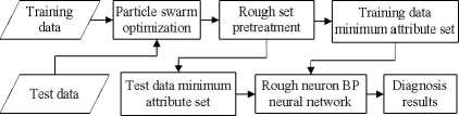
Figure 4. Rough neuron network system.

• B.    Data Discretization and Reduction

In large rotating machinery, rotor imbalance is a kind of common faults. A turbine fault diagnosis example is presented in [20], there are 11 symptoms, using “trainingtest” method, divides given data set into training data set and test data set (respectively random distribution according to 70% and 30%). According to section 4 sample data are discretized with particle swarm optimization. A decision table is obtained after discretization, as shown in TABLE I , no fault expressed by 0 and fault expressed .

TABLE I.

D ECISION TABLE OF DISCRETIZATION

u	Sh	Synvt-:-m										Fault Ei
		s,	s,	st	S-	S.	S,	8.	8,	S„	S„
1	4	0	0	0	2	0	5	0	0	1	0	1
2	4	0	0	0	2	0	3	0	0	1	0	1
3	2	0	0	0	2	0	5	0	0	1	0	1
4	4	0	0	1	2	0	5	0	0	1	0	1
5	2	0	0	0	2	0	4	0	0	1	0	0
6	2	4	0	4	0	2	2	2	0	0	2	0
7	2	4	0	4	0	2	2	1	0	0	3	0
8	3	4	0	4	0	1	2	2	0	0	2	0
9	1	4	0	3	0	1	2	1	0	0	1	1
10	1	4	0	4	0	4	0	2	0	0	3	0
11	0	4	0	4	0	4	0	2	0	0	2	0
12	0	4	0	2	0	4	0	1	0	0	1	0
13	1	2	0	2	0	0	2	0	0	0	0	0
14	1	3	0	3	0	0	0	0	0	0	0	0
15	1	4	0	4	0	2	0	0	0	1)	3	0
16	1	4	0	4	0	4	0	0	0	0	3	0
17	1	2	0	4	0	4	0	0	0	0	3	0
18	3	1	0	1	1	0	0	0	0	0	1	0
19	4	1	0	1	0	0	0	0	0	0	2	0
20	4	4	0	2	0	0	2	1	0	0	3	1
21	4	4	0	3	0	0	2	1	0	0	2	1

Attribute reduction is deleting the unnecessary condition attribute. Thus after analyzing we get condition attribute in reduction for decision rules of decision attribute. And people hope to get fewer conditions of reduction results if possible or get fewer decision rules. According to the definition of attribute dependability, in the information system the importance of any attribute a∈ C-P is SIG(a, P, D) = γ(PU{a}, D) -γ(P, D) . Visibly if SIG(a, P, D) is greater and P is known, attribute a relative to decision attribute D is more important. Let an information system is S = (U,C U D,V, f) , core attribute set is CORE and attribute reduction set is RED(U) , specific algorithm is as follows:

• (1)    Get core attribute set CORE of condition attribute and the dependability y ₁ of attribute C relative to attribute D .

• (2)    Get the dependability y 2 of core attribute set CORE relative to attribute D . If y 2 = y 1 , then jump (5), else let C ' = C - RED ( U ) .

• (з)    Get attribute importance of each attribute in C ' and sort them by ascending order, maximum in them will be added to RED ( U ) .

• (4)    Get the dependability y 3 of red (U ) relative to attribute D . If y ₃ <  y ₂ , then delete the attribute which is just added to red ( U ) and return (з), else return (2).

• (5)    Delete redundant condition attribute in red ( u ) , at last a reduction can be obtained.

Reduct table 1 by using above method, core attribute set is { S ₇ } , the original decision table of condition attribute can be reduction for { S ₂, S ₄, S ₇} .

In the process of discretization, cut sets of each attribute can be obtained, such as 0.1 is a breakpoint of { S ₇ } , according to the code rule [0.06, 0.10) is class 1 and [0.10,0.34) is class 2. So the actual data should be 1 class 1, or class 2? According to the code rule, it should be for class 2, but if considering the error in data acquisition process, the breakpoint may actually be assigned to class 1. If the collected data meets the following formula: Ц - а\,\в — a <  ^e , where X is actual numerical value, α and β denote respectively numerical value which based on discretization cut sets λ located in upper and lower classes of numerical interval, ε is error rate and ε = 0.05 in this experiment. So after discretization the collected data can be considered two values, not s single value. If it does not meet that error formula, it can be changed into two equal values. Then it will meet the input form of rough neuron. So after discretization 0.1 should be “ 1,2 ”. According to the above method, discrete value of the minimum attribute set { S 2 , S 4 , S 7 } as shown in TABLE П .

TABLE II.

D ECISION TABLE OF REDUCING

и	Syrrptom			Fault D
	s.	S.	s.
1	0	0	5	1
2	0	0	3	1
3	0	0	5	1
4	0	1	5	1
5	0	0	4	0
6	4	4	1.2	0
7	4	4	1.2	0
8	4	4	1.2	0
9	4	3	1.2	1
10	4	4	0	0
11	4	4	0	0
12	3,4	2	0	0
13	2.3	2	1.2	0
14	3	3	0	0
15	3	4	0	0
16	4	4	0	0
17	2,3	4	0	0
18	1	1	0	0
19	1	1	0	0
20	3.4	2	2	1
21	3.4	3	2	1

• C.    Diagnosis Analysis based Rough Neuron Network

• (1)    BP neural network

Number of neurons in neural network hidden layer directly relates to the network performance, BP neural network through the comparison of figure 5 before reduction, when number of neurons in hidden layer is 25, misclassification rate is almost 0;

TABLE III.

D IAGNOSIS RESULT OF MODEL BP NEURAL NETWORK

D U	16	17	18	19	20	21
Y 1	0.0002	0.0000	0.0055	0.0055	0.9880	0.9892

Then Error curve of BP model(Figure 6).

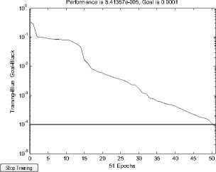
Figure 6. Error curve of BP model

• (2)    Rough set and BP neural network

0.4 0.2

let BP neural network with Rough Sets reduct is model RSBP1 and network output value is Y ₂ ;

BP neural network through the comparison of figure 7 after reduction, number of neurons in hidden layer should be 6.

0V

-0.2

-0.4

-0.6

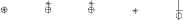
4- number of neurons = 6

*■ number of neurons = 8

number of neurons = 10

-1

12345 | Stop Training |         number of samples

Figure 7. Misclassification rate after reduction

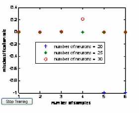
Figure 5. Misclassification rate before reduction.

Let BP neural network without Rough Sets reducts are model BP and network output value is Y ₁ ;

TABLE IV.

D IAGNOSIS RESULT OF MODEL RSBP1

_U 16        17        18        19        20        21

Y 2    0.0000  0.0000   0.0038   0.0034   0.9889  0.9915

Figure 8. Error curve of model RSBP1

• (3)    Rough neuron BP neural network

Let rough BP neural network with rough set reduct is model RSBP2 (shown in Figure.9).

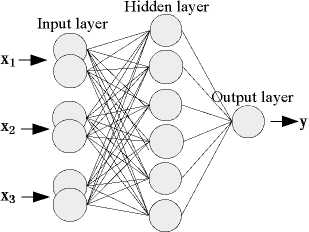
Figure 9. Rough neuron BP neural network

For training sample of No. p ( p = 1,2, ⋅ ⋅ ⋅,P ), Input of No. i rough neuron is property values which is conditional property of No. i in input state of No.

The value is denoted as xpi = (xpi, xpi) .  Then the ouput of No. i rough neuron :

zpi = min( f (xpi), f (xpi))(10)

zpi = max( f (xpi), f(xpi))(11)

Input layer of rough neurons is fully connected with the hidden layer of neurons . So input of hidden layer in No. j :

• rpj =∑n (ωji⋅zpi+ωji ⋅zpi)+θj(12)

i =1

Where ω_ji and ω_ji is the connection weights of lower limit and upper limit , hidden layer of No. j and input layer of No. i respectively.

o_pj = g ( r_pj )                       (13)

Let υ_kj is the connection weights in neuron of ouput layer NO. k a nd hidden layer No. j , θ_k is threshold, Then the ouput of ouput layer No. k :

m ypk = h(∑υkjopj +θk)             (14)

j =1

Where f (⋅) ,g(⋅) ,h(⋅) is transfer function of Input layer, hidden layer and output layer respectively. Let f (⋅) is 1, g(⋅) is function of Sigmoid , h(⋅) is function of purelin .

The network error is defined as:

Pl

E = ¹ ∑∑ ( d pk - y pk )²          (15)

2 p =1 k =1

According to the steepest gradient descent method, the weights is varied along the negative gradient direction of the error function. The correction formula of weight value is derived as :

Ouput layer:	υkj ( t +1) = υkj ( t ) + ηδpkopj	(16)
Hidden layer ：	δpk = ck ( dpk - ypk )	(17)
	ωji ( t +1) = ωji ( t ) + η ' δ ' pjzpi	(18)
	ωji ( t +1) = ωji ( t ) + η ' δ ' pjzpi	(19)
	- rpj       n δ ' = - e       δ υ pj             - r         pk kj 1 + e pj k =1	(20)
Where η , η '	is learning factor respectively

Let network output value is Y ₃ ; so model RSBP2 of actual output as shown in TABLE Ⅴ .

TABLE V.

D IAGNOSIS RESULT OF MODEL RSBP2

D U	16	17	18	19	20	21
Y 3	0.0000	0.0000	0.0000	0.0000	0.9998	0.9998

Performance is 9.49815e-005, Goal is 0.0001

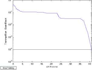
41 Epochs

Figure10. Error curve of model RSBP2

Three models of error curve as shown in figure 7, 8 and 10, obviously model BP neural network reaches minimum error after 51 steps and model RSBP1 reaches minimum error after 34 steps. Both the result completely consistent, but the latter neural network has simple structure, the shorter training. However, model RSBP2 reaches minimum error after 41 steps, although training time between model BP neural network and model RSBP2, its accuracy is higher, fully displays the feasibility of the model of the fault diagnosis.

• V . Conclusion

There are differences between traditional BP neural network and neuronal network that inputs data possessing. Neural network based on rough neurons is proposed in this paper, and given a rough neuron network structure. But due to rough set only can deal with discrete attribute, in the process of continuous attributes discretization, some characteristic data may be classified roughly, not an exact value. If these characteristic data are still taken as traditional BP neural network's input, it has to lose information. Rough neuron neural network compatible with multiple-valued input information by using rough neurons instead of traditional neurons, This also accord with the actual situation. The simulation results show that the complicated network structure leads to the running time of growth, the diagnostic accuracy is higher than the other model.

A CKNOWLEDGMENT

This work was supported by National Nature Science Foundation of Liaoning Province (NO.20071096), Educational Commission of Liaoning Province (NO. 2009A358)