Saint-Venant and Karman equations for an orthotropic pre-stretched plate under tem-perature

Thin plates which are attached to rigid ribs and preliminarily stretched with the help of forces in their plane [1; 2] are used in space technology. Similar are the structures that represent a life net supported by drones to cancel the energy of a person falling from a height for his evacuation both from a high-rise object and in other exceptional cases in the absence or impossibility of using other means of rescue [3].

Composites, often unidirectional ones, are used as material for the plates [4]. Their physical properties sometimes differ by a factor of 15 in two main directions, and strength characteristics differ by a factor of up to 40. Fig. 1 shows the net of a composite plate oriented in the global coordinate system ( Oxy ); the strength parameters with rigidity characteristics in its own main axes O12 are given.

Distributed loads, like local forces, form significant bending moments and shear forces that create stress concentrations [5]. One of the ways to reduce stress is to stretch the plate with membrane forces applied along the contour. If the membrane forces themselves are functions of the transverse load, then the additivity principle does not apply [6]. Uneven temperature loading changes stresses and deformability.

The works [6–11] give the theory of bending of isotropic plates; the works [12–18] present the review and analysis of deformation models.

Purpose of the work . It is required to choose a model for calculating thin plates made of an orthogonally anisotropic material to ensure rigidity and strength under the simultaneous application of transverse and longitudinal loads, taking into account the temperature increment.

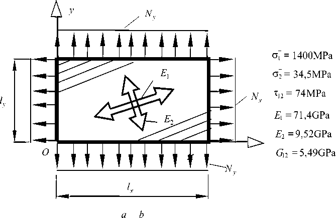
Fig. 1. A net of orthotropic material stretched over a rigid contour:

a - stretching forces N_x , N_y ; b - strength parameters ст + , ст + , т₁₂ and rigidity characteristics E j, E ₂, G₁₂

Рис. 1. Полотно из ортотропного материала, натянутое на жесткий контур: а - силы натяжения N_x , N_y ; б - прочностные параметры о + , ст + , т₁₂ и характеристики жесткости E , E , G

1. Statement of the deformation problem of an orthotropic model of tension and bending

We use Hooke's law for a body with orthogonal anisotropic properties, composed in the Oxyz co-

ordinate system [19] as defining equations:
exx    Г 1/ E 1     -v 21/ E 2     0   1|ст x    fa 1 T
* e yy f = -V 12 / E 1     1/ E 2       0    jCT y Ыа 2 T e          0          0      1/ G12   t        0 e xy J   L                            12 J [ т xy JI	■,                             (1)

Here E 1 , E 2 , v ₁₂, v ₂₁, G ₁₂are elastic rigidity characteristics (technical constants) of the orthotropic material determined for the main directions of elastic symmetry 1–2 ; e_xx , e_yy , e_xy are the deformation tensor components; ст x , ст _y , т xy are the stress tensor components; a ₁, a ₂ are the coefficients of linear thermal expansion of the orthotropic material along the directions of elastic symmetry 1–2 ; T = T ( x , y , z )is the temperature increase. The method of taking into account temperature changes is known as the “deformation elimination method” [9; 10]. In this method, for isothermal loading, volumetric and surface forces are determined through the temperature field T ( x , y , z )of the original temperature problem.

Equations (1) in inverse form have the form

ax 1  Г E1   E12   0 ° у|=Е12  E2    0 1т xy J   [ 0     0   ^12. exx  a1T к-а 2 Н,                 (2) .    exy where the rigidity coefficients are denoted by the following symbols:

E 1        E               F     ^V 21 E 1  -  ^V12 E 2

,   ^ 2 —            ,   E 12 —           —            .

^{1 -V} 12 ^V 21          ^{1 -V} 12 ^V 21           ^{1 -V} 12 ^V 21    ^{1 -V} 12 ^V 21

The theory of deformations, “corresponding to any displacements, not only to small ones”, is applicable from [12]. To calculate the elongation s_V of the considered point in an arbitrary direction v determined by the direction cosines l , m , n ( l ² + m ² + n ² — 1 ), the deformation tensor components have the form

⁸ j ^—

+

^c x j-    ^{d x} i J

d u k d u k

. d x_i d x j

Here u 1 — u , u ₂ — v , u 3 — w are the projections (components) of the displacement vector.

Regarding the application of equations (4) to the bending of plates, we cite the remark of P. Papko-vich: “In the problems of bending thin plates, the deflections of the middle surface w — w ₀( x , y ) are so significant that the squares of the angles of rotation ( d w ₀ / d x ) 2 and ( d w ₀ / d у ) 2 are quantities of the same order as membrane deformations of the middle layer д u ₀ / д x and д v ₀ / д y ” [6 ]. Hence, for the model of a bending flexible plate, equations (4) are taken as follows:

д u 1 f д w ^

8^ —--+----- xx дx  2 кдxJ

,

д v  1 1 д w |         д u  д v  d w S w

—1,  8^, —11, ду  2 К dy J ^  ду  dx  dx ду

d w       d u   d w       d v   d w

----,   8 _xz —--1-- ,   8 _yz —--1-- . д z        д z  д x    ^y   dd  ду

Application of the Kirchhoff hypothesis

8 zz — 0 , 8 xz — 0 , 8 yz — 0 , gives

w ( x , у , z ) — w o( x , у ,0) — w ,   u ( x , у , z ) — u 0 - ^{d w} 0 ( ^x , ^y ) z ,   v ( x , у , z ) — v 0 -d w l xy ) z .     (7)

d x                       д у

Here - h /2 <  z <  h / 2; h is the plate thickness; u ₀ — u ( x , у ), v ₀ — v ( x , у ) are membrane displacements of the middle layer of the plate (at z — 0 ); w — w ₀( x , у ) is the deflection function.

Substituting (7) into the first three equations (5), we get:

xx

d u ₀   д ² w ₀    1 Л d w ₀

d x   d x²     2 К d x

yy

д v ₀   d ² w ₀    1 f d w ₀

д у   д у ²      2 ^д у _?

_{£  =} ^{д u} 0 ₊d v 0_2 ^{д 2 w} 0 ~ । ^{d w} 0 d w 0

^xy   д у   д x    д x д у     д x  д у

.

We set the temperature distribution over the thickness as a linear one:

T ( x , y , z ) = T c + Т h z ,    - h / 2 <  z <  h / 2.

Here the functions

Т c = [ Т ( x , y , h /2) + T (xx , y , - h /2) ] /2,   T h = [ Т ( x , y , h /2) - T ( x , y , - h /2) ] / h        (12)

depend on the temperature increments specified on the front surfaces of the plate.

Internal force factors, which are membrane forces N_x = N_x ( x , y ), N_y = N_y ( x , y ) and S xy — S xy ( x , y ), bending M_x = M_x ( x , y ), M_y — M_y ( x , y )and torque H xy = H_yx ( x , y ), are calculated by integrating equations (2) over the thickness h :

N_x = h ’

E

d u_n   1 ( d w ) 2

—0 + -I — I dx   2 {dxJ

—

^a 1 T c

⁺ E 12

d v^   1 ( d w I ²

—0 + - — | dy 2 ^5y J

—

^a 2 T c

,

N y = h

E ₁₂

M x

M y

d u_n   1 ( d w

0 + -I d x   2 Id x

-a T

+ E ₂

d v_n   1 ( d w I ²

0 + -I dy   2 v dy ?

₇ ( d u_n   d U)   d w d w

Sxv = G12h —0 + —0 +--, xy      12

V d y    d y    d x d y J

I ^d y

h ³

h ³

d ² w

E 1 —+ a T + E

E ₁₂

d x

1 T h

⁽d ² w

^TT ^{+ a} 2^Th

,

(^2wI - ту + aTh+ v dxJ

d_ w j.   т

~y + ^a 2 ^T h

,

H =H

11 xy 11 yx

h ³ _ d ² w

--G 9 --~

6     d x d y

.

Here N x = N_x ( x , y ), N _y = N _y ( x , y ), ..., M_x = M_x ( x , y )... are coordinate functions.

2. The equation of the middle surface continuity

The continuity equations for the middle surface of the plate are formulated as for a plane problem of elasticity theory [16] from equations (8)– (10):

d 2 ^£ xy d 2 e x   d 2 £ y _ d 2 w ₀ d 2 w ₀   ⁽ d 2 w ₀ ¹

— dxdy   dy 2   dx 2    dx 2  dy 2   V dxdy y by elimination of membrane displacements u0 — u(x, y), v0 — v(x, y).

Let us use the “method” from [6], in which the derivation of the continuity equation for an isotropic plate is considered. On the left side of (19), we express the deformations in terms of internal membrane force factors (13)– (15). For this relationship we add (13) to (14) and then subtract them from each other. This will give

V21 txt       xt xdu

---21— (Nx - V,2NV ) —--0 -x12 hE2V12

_V12_( Ny -V 2, Nx )   '  - y

1 V 21                      o x

1 (d w Y

2 v d x J

1 Id w I

2 Y y J

—

a T ,

^-a 2 T c .

We differentiate the equation (20) twice with respect to the coordinate x , and we differentiate (21) twice with respect to the coordinate y , and then we add them. From the resulting expression, we subtract the equation (15), differentiated with respect to the coordinates x , y . We obtain the equation of continuity of the middle surface with respect to three unknown functions N ( x , y ) , N ( x , y ), S_xy ( x , y ) :

^V 21 ^d 2

hE 2 V 12 d y²

( N_x -V 12 N y ) +

^V 12 ^d 2

hE 1 v 21 d x ²

⁽ N y ^-V 21 N x ) ^-

1  d2s   (d2 w У  d2 w d2 w    d2td

—                   --a,   C- -a-, hG12 dxdy  ^5xdyJ   dx2 dy2     dy2

We introduce the Airy function ф = ф ( x , y ) [18] into (22):

i 32ф         1 д2ф   „, 5

Nx = h Д 2 , Ny — h n 2 , Sxy — — h - -

5y2     y dx2

we obtain the desired deformation continuity equation for a flexible orthotropic plate with temperature addition, relative to an unknown function ф ( x , y ) :

^V 21 dJ₊

^V 12 ^E 2 ^{d y _}

^{1     V} 21 ^V 12 I ^d Ф      ^12 ^d Ф _

+

I G 12   ^E 2    E 1 Jd ^x d y   E 1 ^V 21 d ^x

'd w I ²   d² w d ² w _   d ² T_c _    d²T_c

Jd x d y ;   d x ² d y ^{2    1} d y ^{2    2} d x ²

For an isotropic plate, assuming E^ — E ₂ — E , v₁₂ — v₂₁ — V and G ₁₂ — E /2(1 + v) , we obtain:

1 ' d ^_ ф     5 ^_ ф    5 ^_ ф^Л

⁺ 2     +Т7

Е ^d y     d x d y    d x J

' d² w I ² d ² w d ² w     d²T_c      d ²T_c

?-“ 1 c -“ 2 c ,

^5 x d y J   d x ² d y ²       d y ²       d x ²

where the parentheses on the left side contain the double Laplacian over the stress function У ² У ² ф ( x , y ).

• 3.    Equilibrium equations for combining bending with the S.P. Timoshenko tension or compression

Here, two possible cases of stress distribution in the plate are distinguished [11]:

• 1)    tensile stresses are small (compared to critical stresses), and it is possible to neglect their influence on the plate bending and to assume that the total stress is obtained with sufficient accuracy if the stresses caused by the tension of the middle plane are superimposed on the bending stresses produced by the transverse load;

• 2)    the stresses in the middle plane are not small and their effect on the bending of the plate should be considered.

We will use fig. 2 to compile the equilibrium equations of an element from membrane forces (in order to coordinate directions and signs). From the membrane forces the stress is distributed uniformly over the thickness h , the equilibrium equation is written without taking into account the curvature of the surface, as for a plane stress state:

dN  dSm

-x +     + qx (x, y) — 0, dx dy

d S xy + N ₊ d x     d y

q y ( ^x , y ) = 0.

Here q _x ( x , y ) and q ( x , y ) are the forces in the basal plane.

The Airy function (23) satisfies equations (26), (27) for q _x = 0 and q_y = 0 .

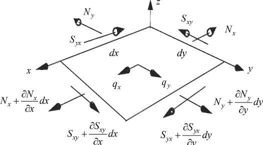
Fig. 2. An infinitesimal element with applied membrane loads

Рис. 2. Бесконечно малый элемент с приложенными мембранными усилиями

The bending force factors acting on the plate element will be considered in Fig. 3. To understand the directions of action of forces and rotations of sections, let us depict a possible curved view in fig. 4. Let's compose an equation for the equilibrium of internal forces of an infinitesimal element of the plate on the axis z :

5 Q       d Q y             (d w

—x dxdy +---dydx - Nxdy sin I — dx        dy               ydx

+ N_x +-- - dx dy sin

x

[      d x     J

(dw d2 w , --i--ddx y dx   dx 2   J

—

⁽ d w I ,

—Ndx sin    + y     [dy J

⁽     , N^N y   Ъ • ⁽d w , d² w , ¹

N „ i--- dy \dx sin-- i-- -dy

[ ^y   d y J     [dy   d y ² ^J

—

I d w | .

— S.,_xdy sin       +

[d y J

d S yx   I

Sm +--—dx dysin yx   dx

⁽ d w y^d

d2 w , dx dydx

+ q z dxdy = 0

We linearize this equation by replacing the sines of the angles with their angles; we give similar terms and discard infinitesimal terms of a higher order of smallness. Then for any inner element dхdy :

dQx  dQ     d2 w  dN dw    d2 w dN dw     d2w  dS dw dS

-+ + —y + Nx—г + —x — + Ny—г + —- — + 2 Sxy---+ —- — + —--+ qz = 0. (29) dx    dy      dx2   dx dx    y dy2   dy dy     y dxdy   dy dx   dx

We add the sum of the moments of all forces acting around the axis y and around the axis x :

Q =d M x i'l l   Q = ^М i H

.

dx    dy      y   dy

We take into account the law of pairing of tangential stresses, which gives H xy = H_yx and S xy = S yx . Substituting (30) into (29), we get:

dX _{+ 2}H^ d x ²      d x d y

^{d 2} M y     d ² w  _M d ² w      d²w

++ N     + N     + 2 S + q — 0.

d y ²      x d x ²     y d y ²      xy d x d y  z^z

M _x

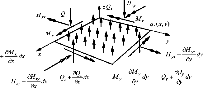
Fig. 3. An infinitesimal element of the basal surface of the plate

Рис. 3. Бесконечно-малый элемент базисной поверхности пластинки

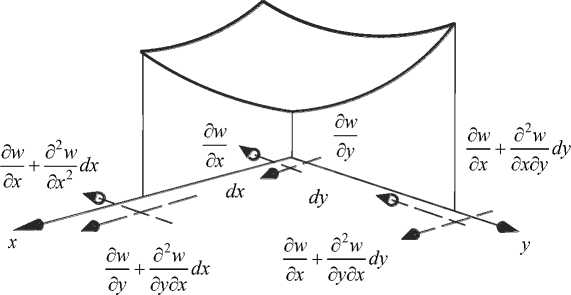
Fig. 4. The curved surface of the plate: the rotation angles and increments of rotation angles in the direction of the axes x and y are given

Рис. 4. Изогнутая поверхность пластинки: приведены углы поворота и приращения углов поворота по направлению осей x и y

Note that equations (26), (27), (31) were obtained without taking into account physical equations (in particular, Hooke's law). It is noted in [7] that the equation (31) was obtained by Saint-Venant (1883).

Substituting the physical relations (16)– (18) into (31), we obtain the B. Saint-Venant equation for a plate made of an orthotropic material:

h ³

\ Ei

^{12(1 -V} 12 ^V 21 ) J

, d⁴ w     d ⁴ w                                  d ⁴ w                 d Th_h

' 1 . 4 + E2 _ 4 +[E1V21 + E2V12 + 4^12(1  V12V21)J -2^2 + E1(a1 + a2V21) _ 2 + dx      dy                               dx dy                dx

\ d2 Th            d2 w     d2 w

+E2(ttiVn + a2) —\ — — qz — N —т— Nv —т— 2S^,---,(32)

• 2   1 12    2 5y2x ax2     y dy2      xy dxdy

• 4.    Classification of thin plates by P. F. Papkovich in connection with the method of their calculation [6]

when exposed to temperature.

Substituting the stress function (23) into (32), we obtain h3

12(1 -v^H

^ Ei

, d ⁴ w    d ⁴ w                                  d w                d Th_h

' 1 . 4 + E2 _ 4 + [E1V21 + E2v12 + 4G12(1  v12v21)j ,2^2+ E1(a1 +a2v21) _ 2 + dx      dy                               dx dy                dx

. a2 t + E 2 ( « 1 v 12 +a 2 ) „ h a y

_     а2 фа 2 w а 2 ф a 2 w    а 2 ф a 2 w ’ = qz   11     tt+ 2        .         (33) a y 2 a x2    a x 2 a y 2     a x a y a x a y

The equilibrium equations (26) and (27) do not need to be taken into account.

The equation (33) and the continuity equation (24) represent a system of partial differential equations obtained by T. Karman. The classical (elementary) theory of rigid plates is a calculation model that reduces to integrating only one equilibrium equation (32).

The theory proposed by Saint-Venant assumes that the plates are thin and the transverse load is so small that the deflections are small. Then, on the right side of (24), the derivatives of the deflection function are small and can be neglected:

1 а ⁴ ф  f 1    „v^ а ⁴ ф     1 а ⁴ ф      a ² t_c     a ² t_c

+ ²^1       += - ^a 1   c -a ₂

E 1 d y   ^ G 12 E 2 Ja x ²d y²  E 2 d x⁴        d y²       d x²

The stress function can be determined from this equation and the boundary conditions independently of the deflection function. Then it is supposed to solve the boundary value problem for (33) with known ф = ф( x , y ) .

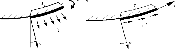
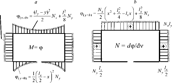
In the case of preliminary stretching of the plate, the function ф on the contour can be calculated using the “frame analogy” [16]. Let the normal c_v h and tangential t_v h components of the stretching forces act on the plate contour separated from the net (Fig. 5), creating a bending moment M = ф in the contour (Fig. 5, a) and a longitudinal force N = d ф / dq (Fig. 5, b). For example, if stretching forces N_x = a_xh , at x = 0 and x = Lx and N-- = 'J-У ■■' у = 0 i\iid у = L. act on the frame (Fig. 1), then the function ф and its derivative can be determined by constructing diagrams of internal forces in the frame (Fig. 5, b and 5, c).

T v h

^ v h

d

c

Fig. 5. The contour of a rectangular plate:

a - the contour element s with the external normal v , in which the bending moment M occurs; b - the contour element s and longitudinal force N ; c - the function ф on the contour; d - the derivative of the function ф with respect to the normal v

Рис. 5. Контур прямоугольной пластины:

а - элемент контура s с внешней нормалью v , в котором возникает изгибающий момент M ; б - элемент конура S и продольная сила N ; в - функция ф на контуре; г - производная функции ф по нормали v

• 5.    Finite-difference statement

Let us replace the plate continuum with a discrete region and differential relations - with finite-difference analogues.

Let us apply central differences [20]. We choose a rectangular uniform grid ® j — { ( x i — i X _x , yj = j X _y ), i — 0,1,..., m , j — 0,1,..., n } on the segments [0, l_x ] and [0, l_y ] on the area of the plate. Here x — x and y — y. are grid nodes; X_x = l_x / m and X_y — l / n are the grid pitch, l_x and l are the dimensions of the plate in the directions of the coordinate axes x and y . The finite-difference analogue of equation (33) is obtained as follows:

a w jj + b ⁽ w jj + 1 + w jj — 1 ) + d ⁽ w j + 1 j + w j-n ) + e ⁽ w j + 1 j + 1 + w j-n — 1 ) + g ⁽ w j + 1 j — 1 + w j — 1 j + 1 ) +

+C(фjj+2 + фjj-2 ) + f(фj+2i + фj-2j) — -qz + k Tjj -1(Tjj+1 + Tjj-1) - m(Tj+1 j + Tj-1 j) , where the coefficients are calculated by the following formulas:

D = h3	/12(1 -v 12 v 21 ), a'		6 DE =  ,    + X y	6 DE xx  +	4 DG 12   2 Nx  2 N y
					x x x y	X2     x y ’
b —- 4 DE x4	_ 2 DG 12 + x x x y	N x , d X 2	4 DE — X4	2 DG  N y 12       y X2X2    X2 , xy    y		DG 12    2 S xy 22         , xy   xy
	g =	DG 12 X2 x y	2 S xy  , 4XX xy	DE 2 f      4 X y	DE , c — X 4	.	(36)

2DE         2DE           DEDE k =  . 2  ((Г +v21a2) + ^T^(a2 +v12a1), l = , 2 («' +v21«2), m = -y2(a2 +v12a1).

X x                  X y                    X x

The finite-difference analogue of equation (24) has the form:

^a ф jj ^{+ b (} ф jj + 1 ⁺ ф jj - 1 ) ⁺ d ⁽ ф j + 1 j ⁺ ф j - 1 j ) ^{+ C (} ф jj + 2 ⁺ ф jj - 2 ) ^{+ f (} ф j + 2 j ⁺ ф j - 2 j ) ⁺

⁺ e ^(ф j +1 j +1 ^+ф j -1 j -1 ^+ф j +1 j -1 ^+ф j -1 j +1 ) =

=------- Г W2,r,i +11'2, , +11'2 T , + W2    +2( —+V —

2л 2       j + 1¹ + 1        j + 1¹ - 1        j - 1¹ - 1        j - 1¹ + 1      '      j + 1¹ + 1   J + 1¹ - 1        j + 1 j + 1   j - 1 - 1

16XVXV L xy

• - wj+1 j+1 wj-1 j+1 - wj+1 -1 wj-1 j-1 + wj+1 -1 wj-1,+1 - wj-1 j-1 wj-1 j+1)] +

• -      ^Г 2 w jj ⁽ - w jj + 1 - wj + 1 j - wj - 1 j - w jj - 1 ) ^{+ 4} w 2- ⁺ w jj + 1 wj + 1 j ⁺ w jj + 1 wj - 1 j ⁺ w jj - 1 wj + 1 j ⁺ wj + 1 w j - 1 j ] ⁺

^X x ^X y

2a,

+1Ji 2+ л 2

^ ^ y^

ji

-^Т+y + Tj-u)-^j + ^-1), ^ y^ where the coefficients are calculated by the following formulas:

6a6a8a        4a    4a        4a 4a       a       a

123         2     3          1     3       2       13

a .4  + ,4  + 2 22 2   ^U       л 4     л 2л 2 , ^U       л 4     л 2л 2 , ^C л 4 , ⁷ л 4 , ^ л 2л 2 ;

^ у ^ x ^ x ^ у        ^ x   ^ x ^ у        ^ у   ^ x ^ у      ^ x      ^ у      ^ x ^ у а, = 1/E1, а2 = 1/E2, 2а3 = 1/G12 -2v21 /E2 = 1/G12 -2v12 /E1.(38)

• 6.    Calculations

• 6.1.    Solution according to the Saint-Venant equation

Plate dimensions:          ,             ; thickness                  . Modulus of elasticity:

E_ = ^CG"2 GPl\ ; £2 = 71.4 GPa; shear modulus G- = "—^] GPa. Poisson's ratios: v₁₂ = 0,02 ; v ₂₁ = 0,15 ( v ₂₁ = v ₁₂ E 2 / E 1 ). The modulus of elasticity E1 is oriented along the long side of the plate, and the modulus of elasticity E ₂ is oriented along the short side of the plate. With this fiber orientation, the orthotropic plate is the most rigid [21].

Coefficients of linear thermal tension of a given orthotropic material: a 1 = 14 - 10 - 5 1/ K (Kelvin), a ₂ = 0.

The system of analytical calculations [22] was used for calculations.

We assume that the pre-stretching forces are known and can be considered constant in the region of the plate and on the contour. Equations (26), (27) are satisfied. In the Saint-Venant equation (32), we transfer the forces N_x , N_y , S_xy to the left side:

h ³

12(1 -v ₁₂ v 2! )

д ² w      d ² w

+Nx —у + Ny —У + 2 SXy x дx2     у ду2      xy

d ⁴ w  _ d ⁴ w

7Г + ^E 2 7Г ⁺ [ ^E 1 ^v 21 ^{+ E} 2 ^v 12 ⁺ 4 ^ 12 ⁽¹

^v 12 ^v 21 ^)]

д 4 w dx 2ду 2

> +

д ² w д x д у

h ³

12(1 -v ₁ 2 v 2 ₁)

. д² T                   д ² T

^E 1 ( « 1 + « 2 ^v 21 ) ХУТ ^{+ E} 2 ^{( a} 1 ^v 12 ^+a 2 ) ХГТ д x                   д у

Now the longitudinal forces are known parameters for the second derivatives of the deflection function and are included in the left side of the system of equations. The transverse load and temperature terms represent the right side of the system of equations. Thus, we have a linear problem with respect to deflection.

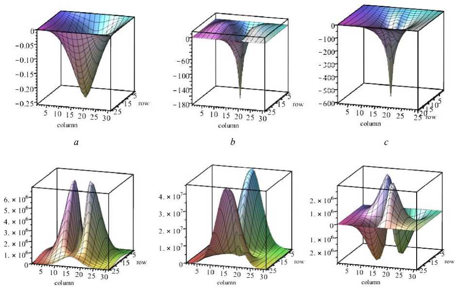
• 6.1.1.    The action of concentrated force

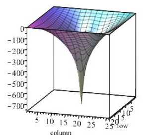
  Let N_x = 0, N_y = 0, Е_лу = 0, T h = 0 . In the center of the plate, we apply a concentrated force P = ЮОО X. Let's replace q z = P /( dxdy ). In fig. 6 we present a diagram of deflections and diagrams of internal force factors. The moments are calculated by formulas (16)– (18). The maximum deflection in the center under the force (Fig. 6, a) is 0.44785 m. The maximum bending moment                     (Fig. 6,

• b ). The maximum bending moment                    (Fig. 6, b ).

Membrane forces are calculated by formulas (13)– (15), however, without taking into account longitudinal displacements:

N_x = h \E_i

1 1 д w

2 < д x

—

a T

+ e ₁₂

1   д w 1

—

^a 2 ^T c

Ny

= h 1 ^ 12

1 ( d w

2 Is x

-a T

+ E ₂

1 (dw 12 2 Idy ,

-a 2 T c

S xy = ^ 12 h

d w d w d.x d y ₎

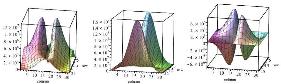
These formulas show that the longitudinal force N_x acquires its maximum value in the region of the plate near the concentrated force P in the direction of the module E ₁ (Fig. 6 d ) , and the longitudinal force N_y acquires its maximum on the contour at the long sides -

(Fig. 6, e ). The diagram of shear forces is shown in fig. 6 e . The forces turned out to be significant,

F A1 (dw 1 ²

, Eh

²  2 ^S y )

.

1 ( d w 1 2

they depend on nonlinear additives: E₁ h — I — I

2 ISx )

Thickening of the finite difference grid in (35), (37) does not change the order of the membrane forces.

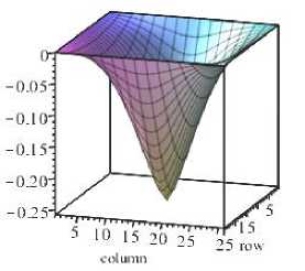
• 6.1.2.    Temperature accounting (Fig. 7)

• 6.1.3.    Action of a concentrated force, temperature and pre-stretching

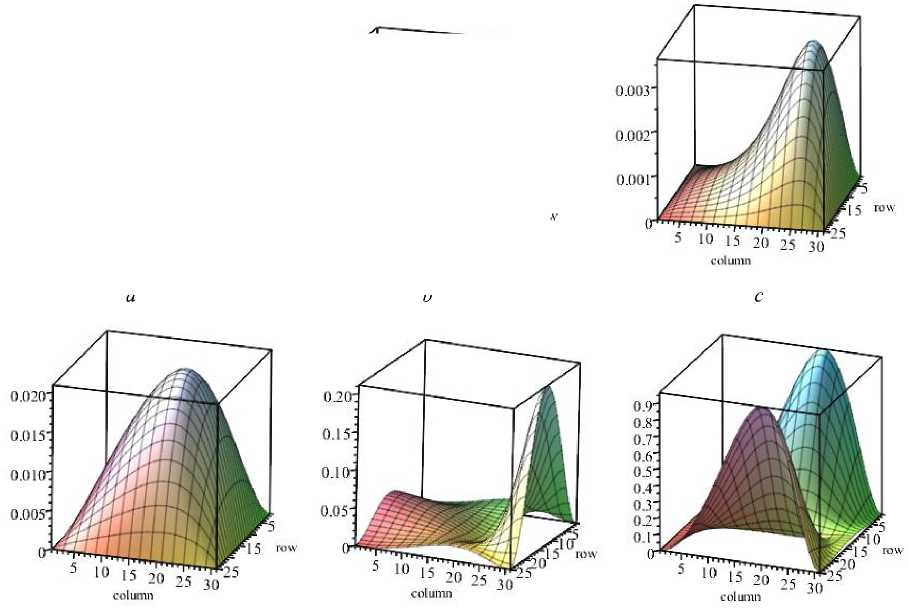
Let us set the law of temperature distribution over the area of the plate in the form T_h ( x , y ) = - 140 o C + ( x / Lx ) 3 80 ^o C . Let us perform the calculations by setting the temperature in Kelvin T h ( x , y ) = 30 K + ( x / Lx ) 3 350 K . The graph of temperature distribution is shown in fig. 7, a . Fig. 7, b–f shows the deflection diagram and the diagrams of internal force factors. Comparing these diagrams with those obtained from the action of a concentrated force, we see that in this flexible plate, with its small thickness, the effect of temperature exposure is insignificant.

The calculation of a thin plate for the action of a concentrated force showed that the resulting longitudinal forces are so large that the stresses are two to three orders of magnitude higher than those allowed for the considered orthotropic material. As it was noted in paragraph 6.1.1, this is the result of the influence of the squares of the rotation angles of the plate middle layer, that is, the squares of the first derivatives of the deflection function. To reduce this effect, one can pre-stretch the plate. Thus, the deflection should decrease, the bending surface will be more monotonous, which should lead to a decrease in stresses.

b

a

c

d

f

Fig. 6. Diagrams in the plate from the concentrated force P = 1000 N:

a – deflection (maximum deflection is 0,44785 m.); b – bending moment М х ; c – bending moment M y ; d – longitudinal force N х ; e – longitudinal force N x ; f – shear force S

Рис. 6. Эпюры в пластине от сосредоточенной силы P = 1000 Н:

а – прогиб (максимальный прогиб 0,44785 м.); б – изгибающий момент М х ; в – изгибающий момент М у ; г – продольная сила N х ; д – продольная сила N х ; е – сдвигающая сила S

Let us add a pre-stretching force (Fig. 8). We obtained a decrease in deflection from the value of 0.44785 m - without taking into account prestressing, to 0.257944 m - taking into account preliminary stretching. The results are presented in the table (lines 2 and 3). Bending moments and longitudinal forces decreased (Fig. 8, b - 8, f ).

If stretches are set simultaneously by forces and , then the maximum deflection will be 0.1864 m; the bending moment , the bending moment . (Theoretically, it is possible to simultaneously stretch the plate in two directions, however, in practice it is difficult to implement).

Once again, it should be noted that, at the prestress of 1 kN/m, in the vicinity of a concentrated force (P = 1000 N) the longitudinal internal forces reach values of the order 4000 kN/m. It can be explained by the presence of a large curvature of the base surface, which is taken into account by nonlin-

,            11 dwY 1 Г 5w ear deformations — —  , — —

2 ^5 x J   2 ^d y

I . Thickening of the finite-difference grid did not reduce this ef- fect. Apparently, two more equilibrium equations (26) and (27) should be added to the Saint-Venant equation in order to calculate the membrane displacements u0 (x, y) , v0(x, y) . Then the deformations du    1 Idw]

\ and —0 + -I — I dx   2 { dx J

.

d v0   1 [ d w will be calculated by the following formulas:--+— —

The simultaneous action of forces                               gives a deflection of 0.27 m (line

• 4 of the table), but does not reduce the deflection. The increase in the longitudinal component by an order of magnitude reduces the deflection by the factor of three (line 5 of the table), however, the stresses do not satisfy the strength. In addition, whatever the transverse load, for sufficiently large values of the longitudinal stretching force, the calculation is reduced to the calculation of the membrane.

  1	Change in deflection and internal force factors	max	Mx	My	Nx	N y	Sxy
  		м	N • m/m	N • m/m	N/m	N/m	N/m
  2	P = 1000 N,WX = 0, Ny = 0	0,448	200	700	12-106	160-106	6 -106

  3	P = 1000 N,Ny = 1000 N/m	0,25	180	600	6 ⋅ 106	40 ⋅ 106	2 ⋅ 106
  4	P = 1000 N,№ = 1000 N/m	0,27	160	600	4 ⋅ 106	50 ⋅ 106	2 ⋅ 106
  5	P = 1000 N,Ny = 10000 N/m	0,0803	140	400	3 ⋅ 106	0,4⋅10 6	1 ⋅ 106

• 6.2.    Calculation using Karman equations

Let us write equations (24) and (33); we apply the iterative method for solving the system of equations.

Option 1. At the first iteration in equation (24) we accept w ( x , y ) = 0 (any approximation is possible). We solve a plane problem of elasticity theory. We substitute the found stress functions into equation (33) and solve the problem of plate bending. The resulting deflections w ( x , y ) are again substituted into the right side of equation (24). We repeat the iterative procedure.

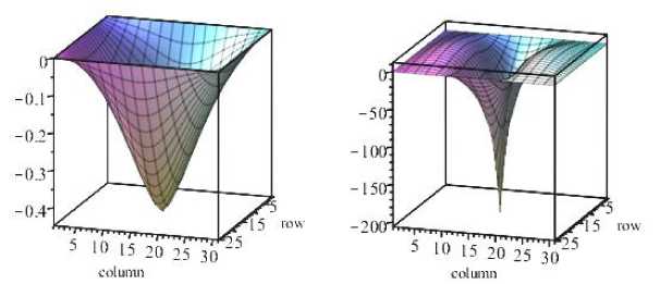
After the first iteration the verification of the solution showed the fulfillment of the equations of continuity of deformations ∇ ² ∇ ² ϕ = 0in all nodes of the finite-difference grid. The deflection (Fig. 9)

was naturally equal to the linear value of 0.257955 m (see line 3 of the table and Fig. 9, a ). Whereas, at subsequent iterations the residuals increased. Solutions cannot be considered correct.

d

f

e

Fig. 7. Diagrams in the plate from the effect of temperature:

a – diagram of the temperature increment (in Kelvin) Δ T = T ( x / L )³ ; b – deflection (maximum deflection 0,000029 m); c – bending moment М х ; d – bending moment M y ; e – longitudinal force N x ;

f – longitudinal force N y

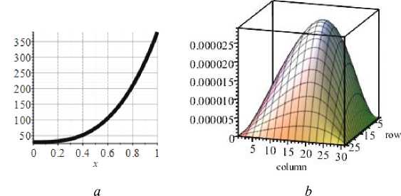
Рис. 7. Эпюры в пластине от воздействия температуры:

а – эпюра приращения температуры (в Кельвинах) Δ T = T ( x / L )³ ; б – прогиб (максимальный прогиб 0,000029 м); в – изгибающий момент М х ; г – изгибающий момент М у ;

д – продольная сила N х ; е – продольная сила N у

Option 2. If we start the calculation with the equilibrium equation (33), assuming in its right side ф ( x , y ) = 0, then the membrane forces are equal to zero. We have a model of rigid bending of the plate; the deflection is 0.44784 m (line 2 of the table for ). The deflection function found is substituted into equation (24) - we obtain the solution ф ( x , y ) . The diagram of the calculated membrane forces as a function of stresses is shown in Fig. 9, b.

The next iteration in this calculation option is essentially a transition to option 1.

The lack of convergence of solutions can probably be explained by the fact that in the equilibrium equation (33) the rigidity matrix has the order 10 ⁶ , and the continuity equation (24) contains coefficients of the order 10 ⁶ - the system of equations becomes ill-conditioned. The problem is non-linear, therefore, to ensure convergence, an increment in load should be applied. Then the discrepancy f of the continuity equations f = У ² У ² ф decreases.

“The apparatus of Karman's theory is relatively very complicated. The complexity and cumbersomeness of the numerical calculations associated with the solution of equations (24), (33) explains the relatively small number of solutions brought to the numerical end in the field of the theory of these plates” [6].

V. V. Novozhilov relates the Karman formulas to an intermediate case between the classical theory of weakly curved plates and strong bending of plates [8].

-300-

-4(ИГ

-5(Xt

d

f

e

Fig. 8. Diagrams in the plate from the action of a concentrated force, temperature and pre-stretching force N y = 1000: a - temperature increment diagram (in Kelvin) AT_h = T_h ( x / L_x) 3 ; b - deflection (maximum deflection 0,000029 m); c – bending moment М х ; d – bending moment M y ; e – longitudinal force N x ; f – longitudinal force N y

Рис. 8. Эпюры в пластине от действия сосредоточенной силы, температуры и предварительно растягивающей силы N y = 1000:

а - эпюра приращения температуры (в Кельвинах) AT_h = T_h ( x / L_x ) 3 ; б - прогиб (максимальный прогиб 0.000029 м); в – изгибающий момент М х ; г – изгибающий момент М у ; д – продольная сила N х ;

е – продольная сила N у

a

Fig. 9. Diagrams obtained by solving Karman's equations: a – deflection diagram; b – membrane force diagram N y

b

Рис. 9. Эпюры, полученные решением уравнений Кармана: а – эпюра прогиба; б – эпюра мембранной силы N y

Conclusion

The calculation of a thin plate for the action of a concentrated force showed that the resulting longitudinal forces, which depend on the squares of the first derivatives of the deflection function, are so large that the stresses are two to three orders of magnitude higher than those allowed for the considered orthotropic material.

With the simultaneous action of a transverse force and a surface stretching load, the deflection decreased by 80%. The bending surface becomes more monotonous, which led to a decrease in the maximum bending moments by 11 and 14%, respectively, across and along the reinforcing fibers of the composite, and the longitudinal forces decreased by 2 and 4 times.

Comparison of calculations obtained from the action of a concentrated force and a change in temperature showed that in this flexible plate of small thickness, the effect of temperature exposure is insignificant.

The apparatus of the Karman theory is relatively difficult to implement numerically. A simple iterative process of solving a system of equations in a mixed form did not lead to the convergence of the deflections and the stress function. The mixed model in stresses and displacements requires additional convergence studies, for example, the application of relaxation methods.

The Saint-Venant deformation model, as a model of a flexible plate with a controlled deflection, allows solving the problems of ensuring the rigidity and strength of the longitudinal-transverse bending of orthotropic plates used in engineering.