Scale Adaptive Object Tracker with Occlusion Handling

Published Online January 2016 in MECS

Due to its ubiquitous applications such as automated surveillance, traffic monitoring, human identification, human-computer interactions, vehicle navigation, aerospace applications etc, object tracking is considered as a cardinal task in the field of computer vision [1]. Despite the advancement of technology, several challenges are encountered in real time visual object tracking [1] [2], such as change in illumination, partial or full object occlusions, complex object shapes, noise in images, scale change, similar objects, cluttered background, real-time processing requirements etc making the design of a perfect algorithm virtually impossible. Evidently constraints, depending on the application, need to be maintained in developing object tracking algorithms solving some challenges while compromising some.

People have come up with numerous visual object tracking algorithms [1]  [3]. Few of them primarily include three steps: (a) extracting features of the object of interest in the initial frame of a continuous video stream, (b) detecting object in the successive frames by finding object of similar features, (c) tracking detected object from one frame to another. Mean-shift algorithm[10] [12], which comprises all of the above mentioned steps, is used as object tracker for the rest of the discussion due to its simplicity and efficiency for implementation in real-time tracking [1]  [2]  [3]. Mean shift algorithm is a nonparametric density estimator which iteratively computes the nearest mode of a sample distribution [4] [11]. It considers that the input points are sampled from an underlying probability density function. It starts with a search window that is positioned over these sample points which continuously moves till the centre of this window coincides with the maxima of that distribution.

But when the object is scaled in any sense with respect to the camera view, classical mean-shift still using the previous window size fails to correctly identify the object. Unlike CAMSHIFT [5] which uses moment of weight images determined by the target model and SOAMST [6] using moment of weight images determined by both target and target candidate model to determine the scale changes, the proposed algorithm uses log-likelihood function to extract only the objet pixels from the infelicitous sized search window and thereby estimating the scale of the object and updating the search window size. But this procedure can be applied only when most of the object pixels are found inside the search window or in other words the mean-shift should be converged.

Again mean-shift fails when the object is taken out of frame or occluded by any other object during tracking. Thus handling occlusions and estimating the scale of the object when the mean-shift is not converged becomes a matter of concern. This paper proposes the use of radial basis function neural network for solving these issues. Applying Extreme learning machine algorithm [7] to RBF neural networks [8] [9] has been proved to provide good generalization performance in most cases and learn faster than conventional algorithms. Thus, several search regions are formed wisely depending on the application and the trained RBF NN is used to identify the presence of object pixels in these regions. In this paper, only RGB values of the object pixels are used as features while this selection actually depends on the computational complexity and accuracy required by the application. The proposed solution incurs reduced computational load and is promising for real-time applications.

The remainder of the paper is organized as follows: Section II describes the overview of proposed tracking algorithm (illustrated in Fig.1). Section III describes radial basis function network for handling occlusions and improving efficiency. The experimental results and comparisons are explained in Section IV and discussions and conclusions are given in section V.

II. System Overview

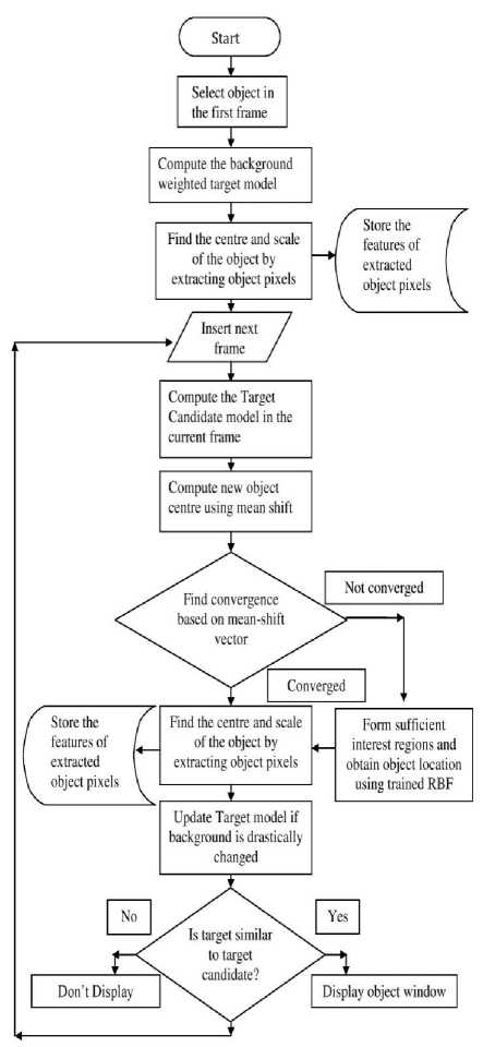
Fig.1. Process Flow of the Proposed Method

feature of all the pixels in the rectangular window is extracted. Feature extraction is the one of the most computationally expensive step in object tracking. Features represent the object and evidently extracting more features will more accurately represent the target object for tracking. But cognizant of the fact that extracting more features will impart computational load and the prime motive of the proposed algorithm is to handle occlusion and being robust to scale change in real time, pixel based colour features is used in the form of R-G-B paradigm.

Now we divide each channel of RGB colour space into k bins or intervals, each constituting an element of the feature space. So we get a feature space vector of к³ bins or elements. Then we find the correspondence of every pixel to the bins so constructed and prepare a histogram.

The colour histogram formed using all the pixels within the rectangular window is used to represent the target. The target model [10] [11] and [12] is given as:

̂={̂ }u=i … (1)

̂ = ∑7=1 к (‖ Xi ‖²) 8 [ b ( Xi )- и ] (2)

Where q̂ is the target model, ̂ is probability of utk element of ̂ , 6 is the Krnocker delta function, b(xt ) associates the pixels xt to histogram bin, к is an isotropic kernel profile, and constant c =1/∑ ^k (‖Xi ‖2) .

The target model always consists of background features. When the target and background are more similar, the localization accuracy of object will be decreased and finding new target location becomes difficult [11]. To reduce the interference of salient

background features in target modelling, a representation model of background features is separately built and the target model is updated based on the background model [11] [12].

The background is represented as {̂} …․ with ∑l ⁼ l̂ =1 in [11] [12] and is calculated by surrounding area of target with appropriate window size

Denoted {̂}U=1 …․  .

by   ̂∗ is the minimal non-zero value in

The coefficients

^{ V_U=min. ^̂ _̂ ^∗ , 1/}

are

used to define a transformation between target model and

target candidate model which reduces the weights of

those features with low V ,i.e., the salient features in the background [11]. Thus the new target model becomes

A . Object selection and Features extraction

The object to be tracked is selected manually in the first frame by specifying a rectangular window. Then the

̂ =     ∑ ^k (‖ Xi ‖²) 6 [ b ( x_t )- и ]      (3)

Where constant C =1/∑ i=l к (‖ Xi ‖²) 8 [ b ( Xt )- и ]

The target candidate model is constructed in a similar way as that of target model but with increased window size as follows

^р (У) = {^GO^l...™            ⁽⁴⁾

й , (У) = С_££^/с(||^||²)^^^     (5)

Where р(у) is the target candidate model, pu(y) is probability of u£h element of p (y), [xj1=l_inh are the pixels in the target candidate region centred at y, h is the bandwidth, and the normalized constant c. ^/sMM2).

Here the target model alone is updated based on background information and not the target candidate model according to [11].

• C.    Extracting object pixels

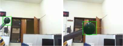
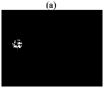
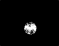
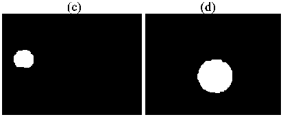
The background weighted target model reduces the weights of salient background features and helps in reducing the background interference in target model. This target model along with background histogram is used to separate the object pixels form background pixel. The log-likelihood ratio of object-background region is used to determine the object pixels as done in [8]. Fig.2 describes the process.

(b)

(e)

(f)

Fig.2 (a), Fig.2 (b) Shows the Actual Tracked Images. Fig.2 (c), Fig.2 (d) Shows the Likelihood Maps “L”. Fig.2 (e), Fig.2 (f) Shows the Morphologically Transformed Images.

For every pixel in the background window, the loglikelihood ratio is obtained as

L = ^«10^/        (6)

1      6\max {h^CO, where h0 (i) and hb(i) are the probability of ith pixel belonging to object and background respectively and e is a small non-zero value to avoid numerical instability.

The log-likelihood outputs positive values for object pixels and negative values for background pixels. Any pixel is declared as object pixel if L ₁ > T. For most of our experiments, T was kept constant at 0.8 which gave satisfactory results. This is further improved by applying morphological operations on the obtained likelihood to accurately represent the object pixels and eliminate outliers. Fig.3 offers an overview of the process.

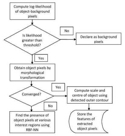
Fig.3. Object and Non-Object Pixel Extraction

• D.    Adaptive scale estimation of objects

The classical mean-shift approach does not estimate the scale of object being tracked neither it adaptively changes the size of search window. In the proposed algorithm, log-likelihood is used not only to extract object pixels but also to address the scaling issues in mean-shift.

After the separation of object and background pixels, we get a rough contour of the object. This outer contour is used for estimating the scale of the object and searching window size (as illustrated in Fig.3 and Fig.4).

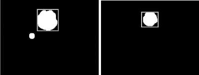
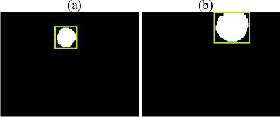
(c)                          (d)

Fig.4 (a-d). Shows the Adaptive Scale Estimations in Frames 10,25,42,68 Respectively.

• E.    Mean shift Tracking

The new target candidate location from the current location is given by mean-shift tracker [11] as

^∑ ГД x_tw_t д (‖ h ‖)

^У‘ =( _∑ ^«18 (‖ h ‖) ⁾

W_t =∑

̂

^{̂ (} ; ) ^5[6( Xl )-^u]

Where g ( x ) is the shadow of kernel profile к ( x ): 9 ( x )=- к ′( x ).

• F.    Background and target updating

The target and the background colour model are initialized in the first frame of tracking. However, the background may often change during tracking due to variations of illuminations, viewpoint, occlusion etc. So there arises a need of updating the background model [11]. First the background features {̂′}    …․ and

{ ̂′}    …․ in the current frame are calculated. Then the

Bhattacharya similarity between old and current background model is computed by

P =∑U = 1 √̂ ̂′ (9)

If p is smaller than a particular threshold, the background model is updated and the target model is also updated based on changes in the background. In the experimental results shown in section IV, the threshold was kept at 0.5. This updating of both target and background model is quite intuitive and helps in improving the efficiency.

• G.    Similarity Coefficient

The Bhattacharya coefficient is usually computed, in tracking algorithms like mean-shift for measuring similarity be tween object and background model, as pB =∑ 11=1 √̂ ̂′ . The target candidate model is constructed from the most recent object centre and an increased version of the updated search window. This increment remains constant throughout the tracking process making the background information interfere more in the target candidate model when the object is scaled down in size. Hence Bhattacharya coefficient diminishes in magnitude when the object is scaled down, not indicating the actual similarity between target and target candidate. So we suggest a modified similarity coefficient based on updated scale of the object as:

Sn = (10)

where s_n is the similarity coefficient and pB is Bhattacharya coefficient between the target and candidate in the ( n -1) th frame, W^ and Wi are window sizes in Tl^th and initial frame respectively. The denominator ^wn in similarity coefficient functions as the scaling factor.

When current window size is equal to the initial window size, the proposed similarity coefficient is just equal to the Bhattacharya coefficient.

When S^ drop below a particular threshold, the algorithm is presumed to be not converged since the target similarity to candidate is reduced as indicated by the similarity coefficient. In our experiments, this threshold was kept at 0.3

• III.    Occlusion Handling and Efficiency Improvement Using RBF NN

The mean-shift tracker basically does the so called “frame to frame” tracking of objects. So it may converge to a local mode or may not converge at all when the object is taken out of frame or occluded in between. It is also prone to local convergence when the object is utterly indistinguishable to the background. The disparate modelling of the target depends heavily on feature selection. Since we are using only RGB features to represent our target, due to various constrained mentioned earlier, we seek the aid of artificial neural network to scout the object in case of occlusion and local convergence.

We initially train the network with different scale and perspective of an object and then use this trained network to search our object when they are abandoned by mean shift tracker. Fig.5 illustrates the training process.

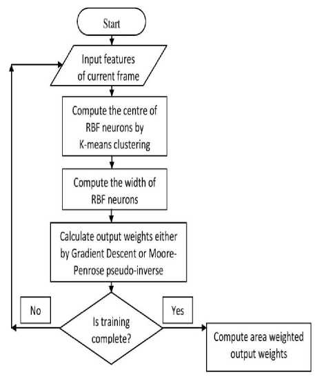
Fig.5. Training RBF Neural Network

Before the usage of RBF NN for our application is elucidated, it is reasonable to discuss the region in which the object is to be searched. When the object is occluded or gone out of frame or not converged, the possible locations at which the object can be seen again are here called as interest regions. The interest region may vary depending on the application, tracking algorithm, the size of object and computational efficiency required. One approach is to divide the entire frame into required number of patches and search for the object in those patches. The patches may or may not be overlapping. Searching object in a greater number of patches makes the algorithm computationally expensive. In our experiments with mean shift tracker, we use appreciable number of patches satisfying both accuracy and time constraint which is explained in section IV.

• A. Radial Basis Function Neural Network

RBF classifier with single hidden layer neurons incorporating fast learning algorithm [7] [8] is proved to approximate any continuous function to desirable accuracy by overcoming many issues such as stopping criterion, learning rate, number of epochs and local minima.

The first layer of the network consists of the inputs which are feature vectors of sample points. We allot first ′ к ′ frames after object selection for the training phase. The exact number of frames required for training phase depends on the accuracy required.

The extracted RGB values of object and background pixels in the previous stages constitute the input signals for our network. So input U is N ∗3 dimensional feature vector where 3 denote the RGB features and N is the number of pixels. The label of each pixel either as object or background forms the output vector Y which is N ∗1 dimensional vector.

The next is the hidden layer which uses Gaussian functions and is non-linear. Each hidden neuron is represented by a centre vector which is one of the vectors from the training set and measure of the width of Gaussian function. The centres can be chosen randomly from the training set. Here we apply K-means clustering on the training set, once for each class and use the cluster centres as centres of hidden neurons according to [13] [14]. Apparently more hidden neurons provide more accurate results but require more computation. K-means is one of the popular and straightforward approaches and is not discussed in detail in this paper. After calculating the centres, the output of each RBF neuron is given as

9j ( U , Cj , Pj )=e Si .‖ U Cj ^{‖ /} ,ј=1…Κ neurons, (11) where ′сj ′ is the centre of j th hidden neuron got from k-means clustering and βj and σj which relate to widths of Gaussian curve is calculated as follows [13] [14]:

σi= ∑ ^1 ‖ Xi - Cj ‖ and

βj 2o"j ² , и ={ ․․ X( ․․ ^N } input data set.

The output of network consists of two nodes one for object and other for non-object. Each node computes a score for the associated class and the input is assigned to the node with highest score. The scores are computed by taking a weighted sum of the activation values from every RBF neuron as follows

К

Ур =∑αjp e  .‖ U-c,   ^, p =1( non - object ),2( object )

In matrix form, Y=Ηα where the dimension of Y, α and H are Ν∗1,Κ∗1 and Ν∗Κ respectively.

These output weights are calculated by Moore-Penrose generalised pseudo-inverse as follows: α=H+ Τ where H+ is the specified pseudo inverse.

The output weights are calculated for input points from each frame till the training phase gets over. At each frame we also calculated the area of objects which is nothing but the total number of object pixels. Then we compute the area weighted output weights α which are presumed to be our finalized parameters for testing phase.

α

∑ L ( A, ∗ a, ) ∑L^Ai

where A i is the area of object and αi is the output weights calculated in the i th frame.

When the object is occluded or mean-shift is not converged by any means, we form interest regions and at each frame, we search the object in one or few of the interest regions presuming that the object movement is not so drastic from one frame to another, until the mean shift is converged.

By searching, we mean that we get features from the current interest region(s) and find object pixels using RBF NN. If the network doesn’t return any object pixels, we shift our interest region(s) until we find the object.

• IV.    Experimental Results

  The algorithm is tested on certain video sequences of 320*240 pixels resolution on MATLAB 2012 environment. A detailed result for ‘blob sequence’ consisting of 334 frames is given below. The object is the dark green coloured circular blob which is manually moved erratically by attaching it to the tip of a rod.

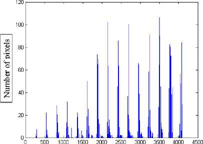
In the first frame, the object ‘blob’ is selected by specifying a rectangular window (green rectangle). Then the RGB features of every object and background pixels are extracted and respective histograms are computed as explained in section II. Here the RGB feature space is quantized to 16x16x16 bins ( к =16) and Epanechnikov kernel is used as kernel function к ( x ) according to [12]. These histograms in Fig.6 and Fig.7 are the RGB based object and background model respectively

Then the log-likelihood function between object and background model is used to estimate the scale changes of the object and the object is tracked by mean shift. The background model is updated whenever there were obvious changes in the background according to [11].

This locates the object more accurately. Some of the frames, where target updating was done, are shown in Fig.8(a-c). During tracking, when the object is occluded or similarity coefficient drops down below a threshold, object pixels are searched in the interest regions. For this experiment, the frame is partitioned into five rectangular areas, one within each of four quadrants and one at the centre and theses areas form the necessary interest regions. Fig.9 shows one such classification by RBF NN into object and non-object at one of the interest regions. Initially, 40 frames are allocated for training for this experiment and the training accuracy of the RBF NN is given in Fig.10.

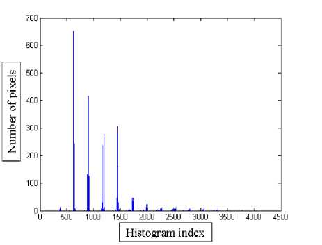
Fig.6. Object Histogram

| Histogram index ]

Fig.7. Background histogram

(a)                     (b)                     (c)

Fig.8. Background Updating At Frames 53(a), 195(b) and 250(c)

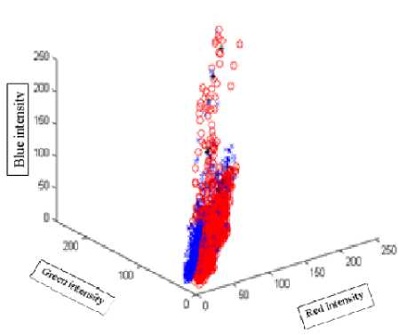
Fig.9. Classification Results of Radial Basis Function Network. Each one of the Three Axes Scales from 0-255 which indicates the Intensity Values of Red, Green and Blue Channels Respectively.

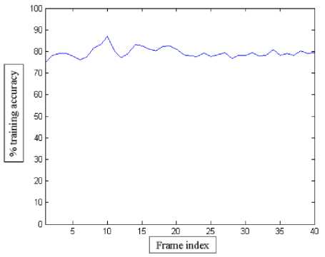
Fig.10. The % Training Accuracy of RBF NN.

The proposed algorithm is then compared with Corrected Background weighted histogram mean shift [11] and Scale and orientation adaptive mean shift [6] algorithms. In [11], a corrected Background Weighted histogram algorithm is proposed where only the target region and not the target candidate region is updated based on background information. Whereas in [6], the zero th order moment and the Bhattacharya coefficient between target and target candidate model is used to estimate the scale and orientation changes of the target.

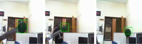
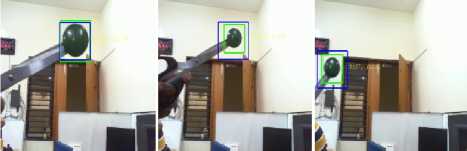
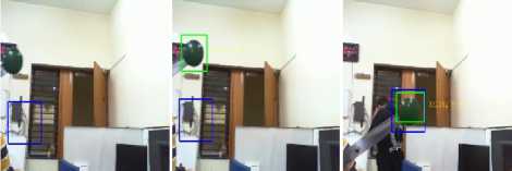
The tracking result of proposed approach and corrected background weighted histogram (CBWH) mean-shift is first showed in Fig.8. Although CBWH does not promise to handle occlusion, the following comparison was carried out to provide a better insight of the proposed method against the most similar CBWH algorithm for object tracking. Object detected by the proposed algorithm and CBWH is shown in green and blue rectangles respectively. When the object is scaled down, the proposed approach identifies the object with correct scale estimation while in CBWH the scale of the search window is unmodified as shown in Fig.11-b. The scale of the object is correctly predicted even when the object is only partially visible as shown in Fig.11-e. When the object is occluded in frame 127 (Fig.11-f), the proposed algorithm rightly reveals the absence of object but CBWH converges locally to the previously found object location. Subsequently the object was found in frame 132 (Fig.11-h) by the proposed algorithm although it missed (Fig.11-g) in frame 130 when the object was first restored in the view. But CBWH identifies the object in frame 195 (Fig.11-i) when the object was brought closer to the locally converged region

(g)                     (h)                     (i)

Fig.11 (a-i). Tracking Results of Proposed Algorithm Vs CBWH Mean Shift for Frames 2, 14 (Object Scaled), 124, 125, 126, 127(Occlusion

Encountered) 130(Object Missed) 132(Object Detected Again By Proposed Algorithm), 195(Object Detected By CBWH).

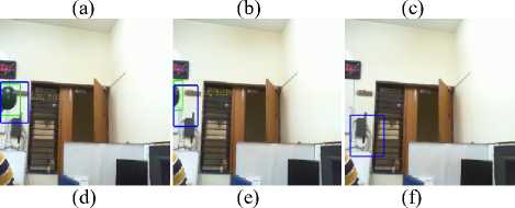
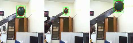
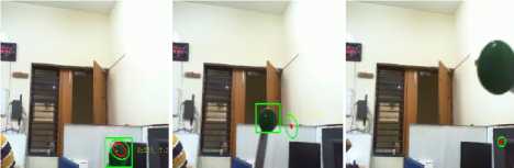
The next comparison was carried out between the proposed approach and the SOAMST [6]. Object detected by the proposed algorithm and the SOAMST is shown within the green rectangle and red ellipse respectively. The green ellipse just represents the background window of the object, according to SOAMST. In [6], the scale and orientation changes of the target were successfully estimated. However, the algorithm worked slowly compared to the proposed one since the former involves heavy computation calculating moments of weight images. When the object is scaled up or down or changed in orientation, it is well tracked by both SOAMST and proposed algorithm as shown in

Fig.12 (a-c). But when the object is moved fast in frame

100 (Fig.12-e) or its background is abruptly changed in frame 85(Fig.12-d), SOAMST was unable to track the object while the proposed algorithm successfully did in most of the conditions. SOAMST remained locally converged till the last frame (Fig.12-f).

(a)                    (b)                   (c)

(d)                   (e)                    (f)

Fig.12 (a-f). Tracking Results of Proposed Algorithm Vs SOAMST for Frames 1, 15 (Object Scaled Down), 25 (Object Scaled Up), 85 (Background Change), 100 (Object Moved Fast) and 265(Local Convergence of SOAMST).

Apart from the above comparisons, the number of iterations taken by the proposed algorithm and SOAMST are compared below for better clarity (Table 1). It can be noticed that from frame 1 to 100, during which the object is clearly observable and scaled at some instances, the proposed algorithm tracks the object with a minimum number of iterations than SOAMST. Thus, it incurs less computational load than SOAMST to adaptively estimate the scale of object making it more favourable for realtime applications. After 100 th frame, the object remained occluded a number of times and for every such occurrence the iterations number reach a maximum for the proposed method while it is unpredictable for SOAMST as shown in Fig.13 and Fig.14 respectively due to local convergence.

Table 1. Mean and Standard Deviation (of Iterations) of Proposed Method and SOAMST are Tabulated for (1) Entire Sequence, (2) Frames 0-100 When the Object is Scaled and Observable and (3) Frames 100-334 When the Object Remains Occluded in Some Frames.

Frame Range SATOH SOAMST Mean STD Mean STD 0-100 3.1900 1.0512 5.1400 2.5585 100-334 2.7094 0.9941 4.3419 3.3601 0-334 2.8533 1.0337 4.5808 3.0996 note: satoh- scale adaptive object tracker with occlusion handling.

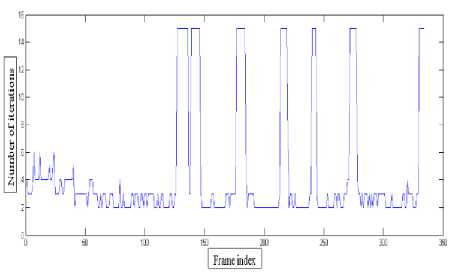
Fig.13. Number of Iterations by the Proposed Method SATOH

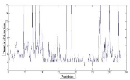
Fig.14. Number of Iterations by SOAMST

The next comparison is carried out between the similarity coefficient as proposed in the paper and the Bhattacharya similarity used in CBWH. The similarity coefficient, correctly predicts the similarity between the target and target candidate when the object is occluded, as nil (as illustrated in Fig.15). But the Bhattacharya coefficient which is used for similarity measurement in [11] predicts the similarity incorrectly in such situations. Further when the object is scaled down in frame 16, the similarity coefficient implies the actual similarity while the Bhattacharya coefficient drops down in magnitude due to scale change (as illustrated in Fig.16).

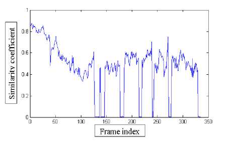
Fig.15. Similarity Coefficient between Target and Target Candidate as Done in SATOH

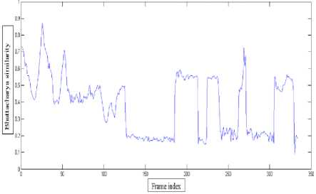
Fig.16. Bhattacharya Similarity between Target and Target Candidate as Done in SOAMST

• V.    Discussions and Conclusions

In this paper, we proposed a hybrid solution to some of the common problems existing in object tracking. The adaptive scale estimation by extracting object pixels and finding abandoned object by radial basis function network incurs less computation burden and hence is more suitable for real-time implementation

The convergence decision in the proposed approach using mean-shift object tracker is based on two parameters-similarity coefficient and restraint on the maximum number of iterations. The similarity coefficient depends on the object to be tracked. If the object is much similar to the background, the decision on similarity coefficient becomes difficult hence local convergence becomes an issue. The maximum number of iterations is again restrained depending on computation constraint. This error can be minimised if more features like texture and shape are used. The decision on search area or interest regions can be tough as even the entire frame can be searched for objects. But due to the computational complexity we restrict ourselves to RGB feature space and limited interest regions.

The proposed method becomes non-parametric by combining neural net with mean-shift and some amount of time must be sacrificed for the training phase and selecting felicitous similarity coefficient for better performance. The algorithm can be improved by efficiently including textures or shapes or other robust features without significantly affecting the efficiency of algorithm to avoid local convergence and intelligently selecting the search region depending on the anticipated trajectory of the object which are currently under our study.

Acknowledgement

We gratefully acknowledge the support from Indian Institute of Science for Scientific Research without which the work could not have been completed. In developing the ideas presented here, we also received helpful inputs on neural networks from J. Senthilnath.