Scale Space Reduction with Interpolation to Speed up Visual Saliency Detection

Published Online July 2015 in MECS DOI: 10.5815/ijigsp.2015.08.07

Region of Interest (ROI) in the image are marked manually or it may be detected automatically from the image features. In general, fast and accurate ROI detection without human interaction is desirable in image processing applications such as object segmentation, object recognition and adaptive image compression. Visually interesting objects naturally draw our attention are called salient objects. The topographical representation of salient objects in an image is called as saliency map. Thus, saliency maps are gray scale images with larger pixel values for more salient points. ROI mask, which is useful in various applications, can then be derived by applying suitable threshold on the saliency map.

Visual salience is the state or distinct subjective perceptual quality which forces some items in the world that pop out from their adjacent items and quickly grabs visual attention [1]. Such as a colorful rainbow in the sky that makes it pop out from its surroundings and draw attention in an automatic and rapid manner. Similarly some parts of the image are more interesting or visually important, that catch visual attention. Thus, salient regions are described as uncommon or unique samples, of the image having distinct features. The regular samples of the image may then be termed as non-salient regions. Computing visual salience has been a topic of interest since last 25 years. Systematic scanning of images from left-to-right and top-to-bottom is the traditional method of attempting to locate objects of interest. Whereas, visual salience provides relatively rapid mechanism to select a few most likely objects and overlook the clutter present in an image [2]. The object scale and their spatial frequencies are associated [3]. Objects in an image become meaningful depending on its scale and distance of observation. For example, a green patch of land in the satellite image may turn out to be a forest in a closer look at the land from an airplane. An even closer look from the top of a building can show constituents of it such as trees, branches, and leaves. The green patch is observed at a coarse scale while the constituents are visible at the much finer scales. Analogous to objects in the real world, details in an image exist over a limited range of resolution. Thus, the concept of scale is very important while processing the image to highlight objects in it. However, scale of salient object in an image is not known in advance. Therefore to detect salient objects accurately multiple descriptions of the image becomes necessary. In the multiple scale analysis, a set of saliency maps is obtained and final saliency map is selected based on minimum entropy value. Scale space or the set of saliency maps is proportional to the size of the image, for example in the case of 128X128 and 256X256 size images the scale space used is 8 and 16 respectively. These multiple descriptions of the image are computationally complex and makes the saliency detection slow.

In the literature, saliency detection is done in different ways. Using simply the low-level image features such as intensity, contrast, color and orientation called bottom-up saliency detection or using some kind of task such as face recognition called as top-down saliency detection. Topdown saliency detection is much slower than bottom-up saliency detection [4]. Bottom-up saliency detection may be of spatial biological, computation or hybrid type. Frequency domain computational models of saliency detection are comparatively fast. Hence, frequency domain saliency detection models are becoming popular. Still they are not either not fast enough to match the requirement of real-time applications or are not sufficiently accurate.

Computationally efficient method called frequency-tuned saliency detection was proposed by Achanta et.al. in [5], which used a bandpass filter of appropriate bandwidth. A saliency map contains the wide range of frequencies, so the wide bandpass filter is formed by combining the outputs of several narrow band pass filters with contiguous pass bands. A wide band filter can include background and noise in the salient region. Thus, to avoid inclusion of background and noise, and to obtain only salient objects, narrow bandpass filters should be used. The accuracy of this method depends on proper tuning of the bandpass filters used, again the question arises how to tune the bandpass filters when the sizes or scales of salient objects are not known a priory.

The state of art visual saliency model of Itti and Koch [6] is a feature integration model. In this model, among all of the chosen features, saliency maps are generated by extracting the feature strength at several scales. The center-surround approach combines them to highlight the salient regions. Then, the individual feature saliency maps are summed to generate a master saliency map. Winner take all stage decides final saliency map. General architecture of this model is a massively parallel implementation to speed up saliency detection. This model forms the basis for other spatial saliency detection models.

SR[7], PFT and PQFT[8], HFT [9] and HSC[10] are the state of art frequency domain saliency detection models. The Computational models of saliency detection employ Fast Fourier Transform (FFT) or quaternion hypercomplex Fourier transforms (QHFT). FFT or QHFT of an image results in the amplitude and phase spectrum. The amplitude spectrum of image consists of all the frequency components present in the image. In the case of HFT model, the saliency map can be obtained by convolution of the amplitude spectrum with Gaussian kernel of a right scale, maintaining the other information unchanged. Fast and accurate saliency detection is the requirement for real-time applications in which ROI is used for further image processing. Scale space reduction is the solution to this problem, but it may affect the accuracy of the saliency map. Modules in [11] attempts to reduce the spectral scale space using bisection search, but occasionally the search trap in local minima. Heuristics search modules proposed in [12] is one of the solution to reduce the local minima trap, while it generate and search the saliency maps. This paper proposes a novel method of scale space reduction with interpolation to speed up the visual saliency detection while attempting to preserve the accuracy of saliency model. To demonstrate the concept, the proposed method is integrated with Hypercomplex Fourier Transform based saliency detection of Jian Li et. al. [9]. The reduction in the computational complexity achieved is O(N/2).

• II.    Background

• A. Object Scale and spatial frequency

There is a close relation between the object scale and spatial frequency. In image low frequencies represent large objects and the background of the image; high frequencies define object boundaries; highest frequencies specify noise, coding artifacts and texture patterns; whereas medium frequencies generally represent the most important parts called as visual salient objects. In order to represent objects of different sizes, it is necessary to convolve a given image I(x,y) with 2D Gaussian kernel g(x,y;o). Where, о defines the width of the Gaussian kernel. In statistics, when we consider the Gaussian probability density function, we call it as standard deviation and о² as variance. The series of Gaussian kernels for low pass filter is given by.

g ⁽ x - ’ ^{; CT} ) = ( Лсту

e

Where, the term 1/ ( 2 _nCT ² ) is the normalization constant. With the normalization, the constant integral of the Gaussian kernel over its full domain is unity for every σ. Thus, the amplitude of the Gaussian kernel decreases rapidly with an increase in σ.

The Gaussian scale-space representation, L ( x , у;ст ) is the convolution of the image I(x, y) with Gaussian kernel g ( x , у ; ст ) written as,

L ( x , у;a ) = g ( x , у;a ) * I ( x , у )

Typically, only a finite discrete set of levels of L for ст >  0 represents the scale-space. For, ст = 0 g ( x , у ; 0 ) is an impulse function and L ( x , у ;0 ) is simply the original image. Further, the Fourier transform of Gaussian F(u,v) is also Gaussian, therefore it can generate the linear scalespace representation that too, without introduction of new structures at the coarse scales [13][14][15].

The Fourier transform of Gaussian is given by,

/      _x      (—2л ² (и ² + v ² CT ² )

F ( и , v ) = e ^{(      (}     )   )

As о increases, smoothing of I(x,у) with a larger Gaussian filter results in removing high-frequency details. The object scale and cutoff frequency of low pass or band pass filters are very much related. The fineness in boundaries and the amount of high-frequency details required decides the higher cutoff frequency of the filters. The bandwidth of the filters should be narrow to highlight salient objects; at the same time, it should suppress background, noise, coding artifacts, texture, and repeated patterns. The use of the band-pass filter can also control the lower cutoff frequency to narrow the bandwidth. The larger is the scale of the object; the lesser is the lower cutoff frequency fLC of the band pass filter. For salient object detection, it is necessary to highlight the entire object. For edge detection, fLC is kept high which narrows down the bandwidth [16]. Similarly, a narrow bandwidth is used for corner and interest point detection [17], [5]. Nevertheless, it is difficult to detect the scale of large elongated object. If we know it in advance, segmenting the object can solve the problem to some extent else using all of the low-frequency contents is the only solution.

In fact, there is no way to know a priori what scales are appropriate for describing the objects in an image, hence, descriptions of the image at multiple scales is considered for salient object detection in hypercomplex Fourier transform saliency detection method.

B. Saliency detection using Quaternion Hypercomplex Fourier Transform

Hypercomplex Fourier Transform proposed in [18], [19], overcome the limitation of the traditional Fourier Transform; it can exploit the correlation between the three-color components and process color image in a holistic manner. For color images, to define the Hypercomplex Fourier Transform, the hypercomplex numbers specifically quaternion are used as.

and f are computed from the three-color channels

r , g , b of the image as,

_ r + g + b 2₃

f ( n, m ) = q i + q 2 i + q 3 j + q 4 Ik

Here q_v is scalar part and q ₂ i + q 3 j + q ₄ k is a vector part in which q ₁, q ₂ , q ₃ and q are real numbers and i , j , k are complex operators that obeys,

i ² = j 2 = k ² = ijk = - 1             (5)

And      ij = k , jk = i , ki = j , ji = - k , kj = - i , ik = - j         (6)

Given a hypercomplex matrix f ( m , n ) , (7) and (8) gives the left sided discrete version of the HFT and inverse HFT respectively. Both F_H [ u , v ] and f ( m , n ) are hypercomplex matrices.

,   n - . M - 1 — ^ ⁽⁽ nu V mv

F H ^[ u ’ ^{v ]} = 1^7^^ e NM '' ^{f (} m ’ ⁿ )

V MN n = 0 m = 0

1   N-1- M-1 + ЦП (( nu )+( mv Ц f (m, n) = j=^^ e    N 'IM '' Fh [ u, v ]

MN" m = 0

Where, ц is unit pure quaternion and Ц = - 1 [9].

C. Representation of Feature Maps

The features considered for saliency detection in the HFT model of [9] are intensity and two opponent color space representations. A fourth feature vector of the quaternion can extend the saliency model to incorporate motion in video saliency detection. Feature maps f , f

g + b V r + b ^

2 Л g   2 J

^ r + g

\2-g\-1A

The feature maps describe hypercomplex matrix

f ( m , n ) as,

^{f (} m , n ) = W j f 1 ⁺ w 2 ^f , i ^{+ w} 3 ^f ; ^{j + w} 4 ^f 4 ^k

Where w and f are the weights and the feature maps. In which, f f f are features of the image and f is a motion feature. For the static image, weight of motion feature is set as zero. Weights of image features like intensity f and opponent colors f and f are set as w₂ = 0.5, w₃ = 0.25, w₄ = 0.25  respectively.

Polar form representation of F_H [ u , v ] in (7) is as follows,

F h [ u , v ] = | F H ( u , v )|| e ^{( цф ( u} ’ ^v ) )         (13)

Where ||F_h ( u , v )||, ф ( u , v ) and ц ( u , V ) are called as amplitude spectrum A ( u , v ) , phase spectrum and a pure quaternion matrix or the eigenaxis spectrum respectively. For handling amplitude spectra, rewriting (1) as a series of Gaussian kernels for low pass filter at different scales k :

g ( u , v ; k )

=      ¹     .-( u ²+ v W^{2 k} -V 0 )

V2 n 2 ^{k - 1} 1₀

Convolution of the amplitude spectrum A ( u , v ) with Gaussian kernels creates smooth Spectral scale space (SSS). Л = { Л^ } represents SSS.

Л ( u , v ; k ) = ( g ( .,.; k ) * A ) ( u , v )

Where, k is the scale parameter k = 1,.... K and it is determined by the image size. For given smoothed amplitude spectrum Л k and the original phase and Eigen-axis spectra, (17) perform the inverse transforms to give the saliency map at each scale: S

S k = g * F h

{ л k ( u , v ) e X ⁽ u , v ) }

Here, д is Gaussian kernel at fixed scale. Fig. 1 shows a series of saliency maps S ^ obtained, for Gaussian filtering of a 128x128 image at scales k =1 to 8. On a saliency map, salient regions are in the highlighted form and rest of the map is in suppressed form. It also reveals that when the scale is very small, the information contained in the amplitude spectrum plots retains quite well, but when it becomes very large, the pertinent information is lost [17]. With an expectation that the histogram of saliency map clusters around certain values, its entropy would be very small. With this assumption, in the HFT saliency model the final saliency map S is chosen from the set of saliency maps S k for a specific scale based on minimum entropy.

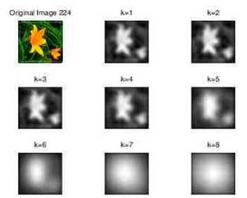
Fig. 1. Image filtered at eight different scales with Gaussian filter.

D. Model Parameters

The comparison of estimated saliency map S and the ground truth map G evaluates the saliency model. By inserting ones at eye fixation locations in a zero matrix, we built a fixation map. Smoothing of the fixation map with a Gaussian kernel produces the ground truth, map. A perfect ground truth map would come from an infinity observers. MIT Saliency benchmark is created from 39 viewers, it has a performance of 0.899 which captures about 95% of ground truth, and is assumed an accurate approximation [20]. To detect salient object regions in a scene, an algorithm should respond uniformly throughout the salient region. Ground truth map segment the entire portion of salient object, hence we use ground truth for comparison.

For analyzing saliency models, we considered more than one evaluation scores to make the conclusions independent of the choice of metric. Area Under the receiver’s operating Characteristics (AUC) and Dice Similarity Coefficient (DSC) measures the performance of saliency detection algorithms and as a measure to evaluate the overlap between the thresholds applied saliency map and the ground truth respectively; The Peak value of the DSC (PoDSC) corresponds to the optimal threshold, and it is the best possible evaluation score [18].

Area under Curve (AUC): To obtain the ROC curve, G and predicted S are converted to binary using fixed and varying thresholds, respectively. ROC curve is then plotted as the true positive rate against the false positive rate averaged over the set of images and over distortion levels, if G e{0-1) , S e{0.1} and the common points of saliency between the two are, A = G n S Equations and (18) compute the True Positive Rate (TPR) and False Positive Rate (FPR) as:

N ( A )

TPR = —

N ( G )

FPR   ( N ( s ) - N ( A ) )

( T ( G ) - N ( G ) )

Where the operator N ( X ) gives the number of ones in X and T ( X ) gives the total number of elements in X . AUC of ROC curve is then calculated [19]. The area under the curve indicates how well the saliency map predicts actual human eye fixations. AUC score of one indicate correct prediction whereas a score of 0.5 corresponds to chance level [21].

Linear Correlation Coefficient (CC) : Pearson's linear coefficient CC measures the strength of linear correlation between two variables

CC ( G , S ) = cov ( G , S ) / ct _g ct _s

Where a_G and a_s are standard deviations of G and S maps, respectively. A CC score of ± 1.0 indicate perfect linear relationship whereas a score of zero correspond to no linear correlation between two variables [22].

Normalized Scan path Saliency (NSS): NSS is the average value of the normalized saliency map at human eye fixation locations [23].

NSS =

N

N p ^{- 1}

s

p

—

M s

^ s

Where the total number of eye fixations is N , the specific location of fixation is p and the saliency map variance is ^ . A NSS score of one indicates that the subject look into the region whose predicted saliency is more than average by one standard deviation, whereas a score of zero corresponds to a chance in predicting human gaze.

Similarity measure (SIM): It measures the similarity between two different saliency maps when viewed as distributions [23]. It is the sum of the minimum values at each point in the distributions. The similarity between two maps S and G is obtained as

X

SIM = ^ min ( S ( x ) , G ( x ) ) x —1

Where

XX

I{ x-1} 5 (x )=I G(x )=1

x - 1                     x - 1

A SIM score of one indicate that the distributions are identical whereas a score of 0.5 corresponds to completely different distributions.

The Earth Mover’s Distance (EMD): EMD is a measure of the distance between two probability distributions over a region [20], [24]. EMD computes the minimal cost to transform the probability distribution of the saliency maps S into the one of the human eye fixations G [25] as:

EMD = min ^fi , j

I f , d , j f i , j

+ I Gi-15j ij

a max d

Where f represents the amount transported from the ith supply to the  jth demand. The ground distance between bin i and bin j in the distribution is d An ij

EMD score of zero indicates that the distributions are identical, whereas a score of one corresponds to no overlap and distributions are completely different [25].

• III.    Interpolation

Interpolation is the process to construct new data points within the range of a discrete set of known data points. Any two points in the plane, ( p , q ) and, ( p₂ , q₂ ) with p 1 ^ p 2 determine a unique first-degree polynomial in p whose graph passes through the two points. It may be generalized to more than two points. For given n points in the plane, ( p_k , q_k ), k = 1, .. ., n , with distinct points, there exist unique polynomials in p of degree less than n that can connect all the points through a smooth curve [26]. This polynomial is called the interpolating function or interpolant. In general, there are three interpolation functions; linear, polynomial and cubic spline for each of the intervals. High-degree polynomials take more time to interpolate. Spline interpolation is used in this algorithm. Spline interpolation uses low-degree polynomials in each of the intervals and chooses the polynomial pieces such that they fit smoothly together. The resulting function is called as a spline. The natural cubic spline is piecewise cubic and twice continuously differentiable. Furthermore, its second derivative is zero at the end points. In this experiment only four saliency maps out of eight are obtained at scales 1,3,6 and 8. At the intermediate scales saliency maps are not obtained, instead they are predicted using the interpolation method. Fig. 2 compares true values of entropy with interpolated values for the two arbitrary sample images imageA and imageB from a MIT database at eight different scales. It is observed that interpolated values of entropy approach the true values of entropy at the intermediate scales 2,4,5 and 7.

Hence, the concept of interpolation is explored to reduce the number of saliency maps in the intermediate stage to make the saliency detection faster. Fig. 3 illustrates the procedure to obtain optimum saliency map with the proposed model. First of all color image is

Original and interpolated curves

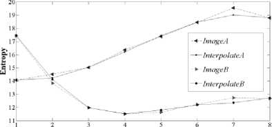
Scale

Fig. 2. Interpolation approach for a sample image from MIT Saliency Benchmark resized to 128X128 to make saliency detection time independent of image sizes. In the second stage, low-level feature matrices such as intensity and color difference are combined to form a quaternion hypercomplex matrix. In the third stage quaternion, Hypercomplex Fourier transform is applied to the quaternion hypercomplex matrix to obtain amplitude spectrum, phase spectrum and Eigen-axis spectrum. With this transform, whole color images can be transformed, rather than as color separated components. These three stages are same as Hypercomplex Fourier Transform (HFT) saliency detection model of [9]. In next stage, Gaussian kernels smooth the amplitude spectrum.

Then, we obtained saliency maps for alternate scales. Entropy is calculated for the derived saliency maps. With the cubic spline interpolation, intermediate entropy values are obtained. Then minimum value of entropy predicts the scale of the optimum saliency map. To verify its correctness actual saliency map and its entropy is derived at the predicted scale. An optimum saliency map with minimum entropy is finally selected. Coding algorithm for interpolation approach is given below.

Algorithm:QHFT Visual saliency with Interpolation Input: The resized color image C with a resolution m x n

Output: Saliency map 5 ( m , n ) of C ( m , n )

Steps 1-3 are according to HFT algorithm of [9].

• 1)    Calculate the feature maps { f ₂, f ₃, f ₄}  form

C ( m , n ) .

• 2)    Combine these features to obtain the hypercomplex matrix f ( m , n ) .

• 3)    Compute amplitude spectrum of f ( m , n ) by

taking its HFT. Preserve the exponential term which consists of the phase and Eigenaxis spectrum.

• 4)    Smooth the amplitude spectrum with Gaussian kernels, according to (2) and obtain saliency maps according to (3) for a specific scale selected by the following interpolation approach.       Let

k = 1, 2, 3... N where N the maximum scale, obtained from image size. For example for images of 128X128 sizes, N is considered as eight.

• i.    Derive saliency maps and calculate entropies for alternate scale for example { 1, 3, 6 and 8 } . This set is called as true saliency set.

• ii.    Interpolate above set to predict entropies at intermediate scales { 2, 4, 5 and 7 } with the cubic spline method.

• iii.    Find the minimum value of entropy E and corresponding scale k .

• iv.    Derive actual Saliency map and its entropy for scale k only if it belongs to interpolated set. Include this saliency map into a set of true saliency maps.

• v.    Final optimum saliency map S is the map corresponding to minimum entropy map from a set of true saliency maps.

• 5)    Return S.

  

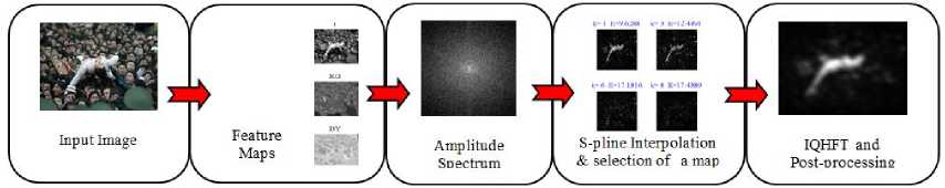
  Fig. 3. Procedure to obtain an optimum saliency map

  true set

  
  

Sample image from MSRA Salient Object Database used in [27] are used to understand the algorithm. Fig. 4 illustrates the progress of the interpolation approach when minimum entropy is part of interpolated set. To verify its accuracy, the actual saliency map is derived at this scale. If the actual entropy found is not a minimum, then the final optimum saliency map is selected from the set of true saliency maps with a minimum entropy value. So in worst case N /2 + 1 is the scale space size. A red border shows the final saliency map, in the Fig. 4. In the second example, after interpolation the minimum entropy found belongs to the true set of entropy. Thus, the saliency map with minimum entropy belongs to the set of true entropy as shown in Fig. 5.

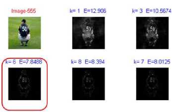
Fig. 4. Progress of interpolation approach when minimum entropy belongs to interpolated set

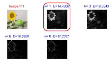
Fig. 5. Progress of interpolation approach when minimum entropy is in

• IV.    Experimentation And Results

  In the experiments of saliency detection in natural images, to evaluate the performance; saliency map S generated by the three state of art saliency models Itti [6], HFT [9] AC [5] and the proposed model are directly compared with the human-labeled salient regions called as ground truth G . The test images and respective ground truth are from the ImgSal V1.0 database by Jian Li [28] which has 235 images of different category. Evaluation is also done with the Achanta’s Salient Object database which has about 1000 images and accurately derived ground truth from the one presented in [29]. For analyzing saliency models, more than one evaluation scores are considered to make the conclusions independent of the choice of metric.

Fig. 6 and Fig. 7 shows the average Receivers Operating Characteristic (ROC) curves plotted as the true positive rate (TPR) against the false positive rate (FPR) averaged over the set of images and over distortion levels, for the proposed and the state of art models of saliency detection. From the figures we can see that, the proposed model HFT-S achived the highest AUC scores of 0.94 and 0.90, for the two databases ImgSal and Achanta respectively and are the same as the HFT model. The ROC curves and the AUC score of this model are better than the other state of art models. In general, the results of HFT and HFT-S models are consistent for the two databases, which proves the reliability of ROC curve and AUC score.

All the models were run on the same Pentium i-V 3.2GHz machine with 3GB RAM. The proposed algorithm of HFTs was implemented in MATLAB 13. The databases, including saliency maps and ground truth for Achanta’s (AC) and Itti’s models were downloaded from the site:

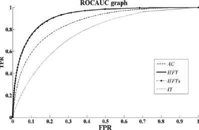
Fig. 6. Area under the receiver’s Operating Curve for ImgSal V1.0 database

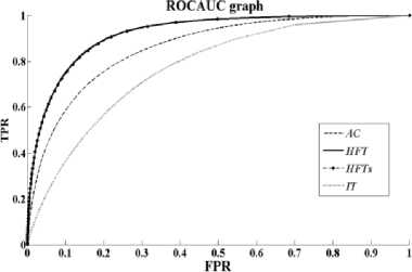
Fig. 7. Area under the receiver’s Operating Curve for Achanta database VPR09/GroundTruth/ VPR09/

The database ImagSal was downloaded from .

Table 1 and Table 2 list the average evaluation scores AUC, PoDSC CC, NSS, SIM, EMD and time to obtain a saliency map of 128X128 resized color images for the two databases ImgSal and Achanta respectively. It is observed that evaluation scores of both HFT and HFT-S are better than AC and Itti. The evaluation scores of the proposed model are close to that of the HFT model. Whereas, the time required to detect saliency is reduced up to half as compared to HFT.

Table 1. Evaluation Scores for Database IMGSAL

Model	AUC	PoDSC	CC	NSS	SIM	Time to compute Saliency map (s)
Achanta(AC)	0.838	0.411	0.46	0.13	0.596	0.032
HFT	0.944	0.587	0.669	0.163	0.6305	0.234
HFT-S	0.943	0.584	0.668	0.163	0.629	0.146
Itti	0.899	0.462	0.518	0.126	0.579	1.1

Similar to HFT, AUC scores of HFT-S is close to one, which indicates the correct prediction of human eye fixation. A CC score of 0.668 indicates a reasonable linear relationship. An NSS score of the proposed method is greater than the other state of the art methods indicates that the subject look into the region. A SIM score of 0.629 indicates that the distributions are almost identical.

Table 2. Evaluation Scores for Database Achanta

Model	AUC	PoDSC	CC	NSS	SIM	Time to compute Saliency map (s)
Achanta(AC)	0.867	0.625	0.456	0.168	0.596	0.032
HFT	0.919	0.691	0.651	0.242	0.640	0.234
HFT-S	0.908	0.675	0.625	0.232	0.629	0.146
Itti	0.776	0.518	0.240	0.093	0.467	1.1

Interpolation approach is also studied for all the six category images of ImgSal database. The Table 3 lists the accuracy of each category. The average scale selection accuracy found is 82%. It indicates that the proposed method is fairly accurate in all the categories of images.

Table 3. Scale Selection Accuracy for Database IMGSAL

Category Salient Region size (Images)	Accuracy Against HFT (%)
Large (1-50)	92
Medium (51-130 )	85
Small (131-190 )	68.33
Cluttered backgrounds (191-205)	86.67
Large and Small (206-220)	93.33
Repeating Distracters (221-235)	86.67

• V.    Conclusion

The scale of salient object is an important factor, but it is not a known priori. In this context, HFT and other saliency detection models use multiple scale descriptions of the image. This paper proposed interpolation approaches to predict the appropriate scale and speed up saliency detection in the framework of HFT model. The interpolation approach only generated alternate saliency maps. Therefore, the proposed method reduced computational complexity from O (N) up to O (N/2) as compared to the HFT method. Scale selection accuracy of this method is about 82%. The performance scores for the proposed model and state of the art HFT model matched with each other. It concludes that the scale selection of the proposed method is not only accurate, but saliency detection is also faster than HFT model. It is worth noting that this method is free from local minima trap.