Seamless Panoramic Image Stitching Based on Invariant Feature Detector and Image Blending

The merging of different images captured from same scene with overlapping regions to form a composite image or segmented panorama is known as image stitching [1]. Typically, cameras have a limited viewing angle compared to the human eye. Therefore, a single picture could not represent the entire region of interest (ROI) of an image due to the narrow field-of-view (FOV) [2]. To overcome this problem, stitching multiple images of the same scene captured from various viewing angles construct a combined image with a larger FOV. Special lenses are used in a camera covering a broad view of an image to create such panoramic images. Unfortunately, the cost of such a lens is very high and practically impossible to use in typical applications that requires wide-angle view or panoramic views. Image stitching is a challenging and promising research area which can be utilized in various fields such as forensic investigation science, image mapping, original data recovery from a damaged image, motion detection and tracking, resolution enhancement, video compression, augmented reality, image stabilization, mosaic-based localization etc. [3]. Image stitching is also difficult in real-time applications like video conferencing, video matting, video stabilization, satellite imaging and medical imaging. In real time applications images can have different depth level, different orientation and varying illuminations [4].

Now commercially available mobile phones have internal stitching facility for panoramic photography [5]. Some devices create panoramic images by capturing images sequentially by moving camera in one direction such as left to right only. But generally panoramic images are composite images constructed from sequences of photographs taken by moving the camera in different directions and orientations. A perfect stitching device should able to stitch these kinds of sequences of images. There are different types of panoramas such as partial panorama, cylindrical panorama and spherical panorama [5]. Partial panorama is a very wide-angle panoramic picture, created by assembling multiple photos of a portion of landscape. Cylindrical panoramic is an image that is meant to be viewed as it seen through inside of a cylinder. We may rotate the image 360 degrees horizontally. Cylindrical panoramic photos are most commonly employed for capturing large open exteriors or interiors with little interest in the floor or ceiling. In contrast, a spherical panoramic image encompasses the full viewing sphere, allowing the observer to look in any direction. A spherical panoramic image is not a three-dimensional image: it is still a single-viewpoint image, but its field of view is unrestricted [2]. Another critical problem associated with the panoramic photo is the presence of a visible seam at the joining boundaries of the stitched image. Identifying the exact matching features and aligning the images based on these matching features are not sufficient for creating a perfect panorama. Therefore, we propose an image stitching method based on invariant feature detector and image blending. Image blending algorithms are applied to eliminate the visible seam across the stitch. Peak Signal [6].

2.    General Methods for Image Stitching

The main steps in image stitching are classified into calibration, image registration and image blending. There are different types of image stitching approaches based on image registration. The different categories of image stitching are direct method also known as pixel-based method, frequency-based method and feature-based method [7]. The goal of image registration is to find the overlapping areas between images and align them as a composite image based on the estimated transformation parameters. In direct image registration, a pixel-wise comparison is accomplished for identifying the similarity between the stitched images [8]. In the frequency-domain-based registration, phase correlation is used for measuring similarity among the stitched images. In feature-based method, feature points/ key points are identified and compared to obtain the overlapping region [3]

• 2.1.    Direct Method

• 2.2.    Frequency-based Method

• 2.3    Feature-based Method

3.    Related Work

The direct method identifies the overlapping areas among the stitched images by comparing each pixel with respect to the source images. One of the main limitations of direct approach is that it could not estimate the pixel-wise similarity while applying scaling and rotation to the input images. Sum of Absolute Difference (SAD), Sum of Squared Difference (SSD), Mutual Information (MI), and Correlation methods are examples of direct similarity measures. These methods can be used for identifying the overlapping region in the images [8].

The Fourier Transform is used in frequency domain image stitching (FT). FT is a two-image correlation that calculates the product of one image's FT coefficients against the complex conjugate of the other [9]. One of the Fourier Transform based image stitching methods is phase correlation-based image stitching. The elementwise product of the input image's Fourier transform with the complex conjugate of the second input image's Fourier transform is used to identify the overlapping area between two input pictures in this method [9]. Image stitching based on cross-correlation can handle both horizontally and vertically misaligned images at the same time [10]. Using phase-correlation based registration, this issue can be solved. Image stitching methods based on phase correlation stitch images with both horizontal and vertical shifts at the same time. On the basis of phase correlation, several image registration algorithms are proposed [9,11]. Fourier-based method is one of such method that is often used to speed up image registration process [8].

Comparing the features of one image against all the features in the other image is an essential step for locating related regions in two images. The key steps of image stitching are feature point extraction, feature point matching, and homography calculation. Features of an image can be points, lines, corners, edges, or any geometric shapes [4]. Featurebased image stitching methods are invariant to scene movements. It also has the capability of identifying the adjacent images among unordered images. Feature-based stitching is computationally faster than direct image stitching methods. The main steps in general feature-based image stitching are depicted in Figure 1. Features detection is considered as the most prominent stage in feature-based image stitching [4]. A local feature detector must meet a number of constraints, including being resistant to image transformation operations such as, scaling, translation, rotation and affine transformation. It also must be resistant to noise, image blur, occlusion, clutter, and variations in lighting, as well as being repeatable. To accurately compute the correspondence between different images, the detected feature points must be represented independently. Real-time image stitching processing involves different stages such as feature detection, description and matching. Corner features leads best feature matching points and that should be matched sufficiently. The most crucial property of a corner is that if one exists in an image, its surroundings will display a sharp change in intensity. Local feature descriptors also define the local content of a pixel in an image. These features are used for image matching of all other images after feature detection. RANSAC (Random Sample Consensus) computes homography H, computes inliers, keeps the largest set of inlier points, and then recomputes the least-squares H estimate on all inliers. Image warping is another important step that digitally manipulates an image to eliminate the distortions in the image [4]. The last process is blending the pixel intensity values in the overlapped region to avoid the presence of visible seams. Image blending is a technique for obtaining a seamless transition between images by changing the image grey levels in the area of a border [12]. The flowchart of the image stitching method is given in Fig. 1.

Various image stitching approaches have already been proposed in literature by many researchers. All these works are discussed and implemented using different image stitching methods mentioned above. As part of this work, some of the feature-based image stitching methods are studied and reviewed here.

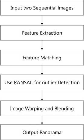
Fig. 1. Flow chart of Image Stitching

In 2017 Maosen Wang et al. proposed a panoramic image stitching method using ORB (Oriented FAST and Rotated BRIEF) algorithm [1]. ORB method is utilized for feature detection and matching, which augment the direction of information to the FAST (Feature from Accelerated Segment Test) detector. Ethan Rublee et al. presented the ORB characterization method. Following that, the RANSAC algorithm is employed to remove any false matching points. Finally, the image fusion is done using the weighted average approach. According to experimental results, the stitching output of the method in this work has the same result as the SIFT and SURF algorithms. The two most evident merits of the proposed algorithm are (1) Speed of stitching, which is significantly faster than other two methods, and (2) Robustness to camera external settings. This proposed method employs FAST as a feature point detector and extracts features in a relatively short amount of time; however, it lacks directional information. The FAST detector is enhanced by the ORB algorithm, which adds direction information (OFAST). The BRIEF descriptor lacks rotation invariance; however, the ORB technique defines the patch moment to achieve a description of rotation invariance. The RANSAC technique removes the mismatched points after extracting the BRIEF descriptor from the main direction. The performance of the proposed stitching algorithm is significantly faster than the other two methods. Three sets of images are used for experiments. In the first test object, SIFT, SURF and ORB takes 24477.472 Milli Seconds, 2344.54 ms and 610.526 Ms respectively.

In 2018 Kyi Pyar Win et al. proposed a method for stitching biomedical images using ORB [2]. The five stages of the proposed method are pre-processing, features detection, features matching, homography calculation, and image stitching. The ORB algorithm is used for feature detection. This method detects feature points with Oriented FAST and generates descriptors with Rotation BRIEF. Unlike SIFT or SURF, the FAST method recognizes features with a single operation. The detection of feature points is done by comparing 16 pixels around the central pixel. This makes the algorithm faster than the other algorithms. Furthermore, the descriptor generated is made up of binary strings. Compared to the SIFT or SURF algorithms, this descriptor uses less memory. The ORB algorithm increases the FAST detector's ability to discern corner orientation. The original FAST detector is incapable of detecting orientation. In the proposed method, nearest and adjacent neighbors of features are identified by calculating the hamming distance. Time consumption of the ORB algorithm is low compared to SIFT, SURF, and Harris corner detectors. The proposed method is compared with SIFT, SURF and Harris corner detector. Total time consumed by SIFT, SURF, Harris corner and ORB algorithms are 8.012932s, 0.65411s, 0.75314s 0.102941s respectively. ORB requires less time to detect features compared to other three methods. Among all the feature detectors, Harris and SIFT detected the most feature points, however SIFT took the longest to analyse. Harris corner detector only works for small changes in Scale and rotation and needs advanced knowledge of window size. It is not scale and affine invariant. ORB detects a smaller number of feature points compared to other methods, but the detected features are relevant and unique. ORB had the least matching time. The proposed method has the advantage of being able to detect accurate key points while also having a lower mismatch rate than other feature detectors. Because binary string descriptors are used, the suggested technique has a rapid matching speed. However, in the case of complicated images, the proposed methods fail to reliably register.

In 2018, Zhang W et al. proposed a remote sensing image stitching for creating a mosaic image based on the SURF algorithm [3]. SURF algorithm is used for extracting features in the input images and creating the corresponding feature descriptors. After the feature points are detected, feature matching is done by measuring the Euclidean distance between two feature points. First, the key points with the shortest and second shortest distances are estimated. The matching is successful when the minimum and second minimum distances ratio is less than the threshold value. Next, the perspective transformation between input images is estimated, eliminating the outliers in the matching point using the RANSAC algorithm. The results reveal that this method enhances the feature point detection matching speed while retaining the SIFT operator's greater registration accuracy.

Zhang T et al. presented a technique for producing a remote sensing image mosaic by utilizing an enhanced SURF [4]. Image binarization is used to perform image pre-processing, feature points are retrieved using a Hessian matrix, and feature descriptions are generated using the circular neighborhood of feature points. The normalized grey-level variation and second-order gradient in the neighborhood are measured parallelly for obtaining a new feature descriptor. The Haar wavelet response is utilized to create feature descriptors. The RANSAC technique is then utilized to remove the outlier points. The standard SURF algorithm has many drawbacks including a large feature vector, expensive calculation and low matching accuracy occurs when both the rotational angle and the viewing angle are excessive. The proposed algorithm improves the SURF feature extraction by eliminating the problems of the traditional SURF algorithm in image stitching. The feature points in the non-overlapping regions are eliminated first. The non-overlapping part's feature points are not only worthless in matching, but they also have an impact on matching accuracy. The classic SURF algorithm finds the similar feature vectors by using Euclidean distance. We can see from the above that the technique generates a 64-dimensional feature vector. The Euclidean distance will become insensitive as the dimension grows, weakening the matching impact and increasing the false matching rate. The proposed method is implemented using ten groups of rock images, each of which is subjected to eight experiments. The algorithm's execution time is calculated and compared. It has been discovered that the enhanced algorithm's efficiency has grown by roughly 17%, and its stitching speed has increased.

In 2021, Yuan Yiting et al. proposed a seamless image stitching technique based on super-pixels for UAV (Unmanned Aerial Vehicle) photos. UAV remote sensing can quickly acquire the most perceptive high-resolution photographs of the target region, providing a precise basis for decision-making. It is challenging to properly capture the entire region of interest from a single UAV photograph, however, due to the UAV's flying height and the digital camera's focal length limitations. In order to swiftly create a high-resolution image with a larger field of view, a succession of overlapping UAV photographs must be combined. They conducted experiments on the new road corridor, airport, and small village data sets to confirm the efficiency of the suggested approach. They proposed a novel superpixel-based seam-cutting method. The proposed algorithm stitches a pair of UAV images. For image registration, the authors employed an adaptive as-natural-as-possible (AANAP) warping method [5]. On a continuous region, the superpixel seam cutting approach is utilized to find an optimal seam. The super-pixel seam cutting method includes three steps such as registration, seam elimination, and blending. In stitching, two warped UAV images are created from the data set by using AANAP techniques. They implemented seam cutting by using super-pixel segmentation to select the best seam and copied each warped image to the corresponding side of the seam. Super pixel segmentation replaces the computationally intensive pixel-based seam cutting method. They also included a cost difference tool, which shows how similar overlapping areas in input photographs or images are. Finally, they combined colour, gradient, and texture complexity to obtain a seam that passed through area with high similarity to avoid conspicuous objects and cross an area with low-texture complexity [16]. Finally, using weighted color blending, the visible seams between the two images are erased. Misalignments and ghosting are challenging problems in image stitching due to large parallax The authors claim that the proposed method is suitable for working with images with significant parallax errors. AutoStitch, DHW, APAP, SPHP, and NISwGSP are a few image registration techniques. In tiny parallax scenarios, registration techniques have produced good alignment precision. Scenes with a lot of parallaxes will show artifacts like misalignment or ghosting.

We analyzed some of the feature-based image stitching works. Features detectors such as SIFT, ORB, Harris Corner detector, SURF, BRIEF etc. are used in the literatures. Some authors compared the performance of these feature detectors [6]. The literature study shows that, while the ORB methodology detects fewer feature points than the SIFT and SURF algorithms, the majority of them are potential key points. SIFT takes a long time to compute, yet it is resistant to image scale, rotation, and light variation. The Harris corner detector has the highest amount of feature points extracted. FAST has been improved and is now faster than ORB, SIFT, and SURF. In FAST, there are a lot of feature points. Some work does not involve seam elimination. So, the final output image shows the stitching line between the boundary area of input images. The seam occurs when the images have large variation in brightness or illumination. Alignment error occurs when the stitching algorithm fails to align multiple images that has huge variation in orientation, illumination and scale. From the analysis of related literature there is scope for enhancing stitching accuracy in all of these feature extraction-based image stitching methods in the future.

4.    Proposed Method

One of the most extensively used image matching algorithms based on image features is the Scale Invariant Feature Transform (SIFT). David Lowe proposed it in the year 1999 [18]. SIFT is both a feature detector and descriptor. The features are scale and rotation invariant, as well as somewhat invariant to illumination and 3D camera viewpoint changes. Furthermore, because the features are unique, a single feature can be effectively matched against a huge collection of features, establishing the foundation for object and scene recognition. SIFT's essential steps are scale-space extrema detection, key point localization, orientation assignment, and key point descriptors [18]. A Difference-of-Gaussian (DoG) function is used to obtain the scale-space extrema points. Candidate key points are localized to subpixel accuracy in the second step and those unstable key points are discarded. The next stage is orientation assignment, which involves creating an orientation histogram to calculate the gradient orientation by sampling the center neighborhood of the key point. SIFT is able to generate a key point invariant to similarity transforms due to the specified orientation(s), scale, and placement for each key point. The final stage is to describe the key points. The gradient magnitude and orientation at each image sample point in a region surrounding the key point position are measured to generate a feature descriptor. The four steps of SIFT are discussed in detail in the next subsection. Unlike Harris corner detector [7], SIFT can perform feature detection independent of the image properties such as viewpoint, depth, and scale.

• 4.1    Feature Detection

The UDIS data set images are color images. In preprocessing stage, we first converted this color images into gray scale images. These converted gray scale images used for detecting feature points. SIFT is used to detect features like corners, circles, blobs, etc. The first step involved in SIFT is scale-space extrema [18], which aims to recognize locations and scales assigned to the same object or scene several times. For recognition, a continuous function of scale using the gaussian function is used to look for stable features over many scales. The scale-space L(x,y, a), of an image I(x, y) is produced by convolving image I(x, y)with a variable-scale Gaussian kernel G (x, y, a) as given in (1).

L⁽x,y,v) = G⁽x,y,v) * I(x,y) (1)

Where о denotes the scale factor that controls the scale and * denotes the convolution operator. A Gaussian function blur or smoothen an image. Gaussian filtering refers to the process of employing the Gaussian function in spatial filtering. It's a technique for reducing image noise [19]. The Gaussian function can be calculated as,

G(x,y,o) =^ ; е ^-(х2+У²^^/2а2 (2)

Where x and y represent the row and column size of the Gaussian kernel and σ denotes the standard deviation of the Gaussian distribution. According to Lowe (2004), smoothing the original image using a Gaussian kernel with о value equal to 0.5 and doubling its size using linear(nearest) neighbor interpolation increases the number of stable features recognized by SIFT [18].

In SIFT, at first image is repeatedly convolved with a Gaussian kernel as given in equation (1), resulting in a series of scale-space images. There are several octaves in the scale space. A sequence of filter response maps is represented by an octave. First, we take the image and perform a blur operation with different sigma values to create the first octave. Then down sample the image by half of its size and also applies different blurring factors for different sigma values to create another octave. The Gaussian blurred image is down sampled by a factor of two after each octave. Each octave is further subdivided into an integer number of intervals. To get the Difference of Gaussian (DoG), subtract the adjacent Gaussians (Difference of Gaussians) separated by a constant multiplicative factor k [18]. The value of each pixel in the D (x, y, a) image is compared with the values of its eight neighbors and its nine neighbors in the images above and below. If the value of a key point is greater than or less than the values of all of its 26 neighbors, it is designated as an extremum (maximum or minimum) point. The difference of Gaussian can be calculated as given in (3), [18]. The DoG calculation is depicted in Fig. 2

D ⁽x, y) = (G ⁽x, y, ко) - G⁽x,y,o)) * I (x, y) = L (x, y, ka) - L (x, y, a) (3)

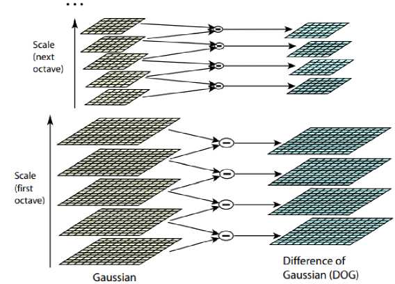
Fig. 2. Set of scale-space(left) and Difference of Gaussian (DoG) (right)

The features with low contrast and features that are located in the corners of the images are eliminated. The next step is to give each key point a uniform orientation for representing a key point in terms of its orientation and so make rotation invariance. In the Gaussian-blurred image, any pixel in a nearby region around the main point has its gradient magnitude and direction. The magnitude of a pixel is determined by its intensity, while the orientation determines its direction.[19].

The gradient magnitude of L(x,y,a) is denoted by m(x,y), and orientation angle is denoted by 0(x,y) . The gradient magnitude and orientation angle are calculated using pixel differences as given in (4) and (5):

m(x,y) = ^L(x + 1,y) - L(x - 1,y))² + L(x,y + 1) - L(x,y - 1))²               (4)

6(x,y),= tan ^-1 (L⁽x,y + 1) - L(x,y- 1))/(L⁽x + 1,y) - L(x - 1,y))              (5)

Each key point has a position, size, and orientation in the key point definition stage. Consider a small area around the key point. Further it divided it into nxn cells, n is the number of cells in each row/column. Each cell is composed of 4×4 pixels. A histogram is created for each of these sub-blocks based on magnitude and orientation [20]. The size of the feature descriptor is rn2. Where r is the total number of bins in the orientation histogram. In SIFT, r=8, n=4. Finally, the length of each feature descriptor become 128 [18]. Fig. 3 shows the process of creating the key point descriptor.

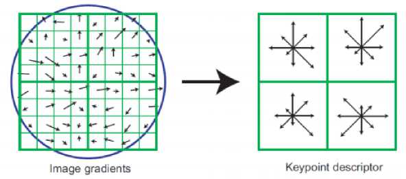
Fig. 3. Feature vector generation

• 4.2    Feature Matching with Brute-Force Matcher with KNN

• 4.3    RANSAC -based outlier detection

  RANSAC is a method for finding the mathematical model parameters from a set of observed data points that to be included as outliers [22]. An outlier can be a measurement variability or it can be an indication of experimental error. Fischler and Bolles proposed the RANSAC algorithm in 1981. RANSAC employs a technique known as repeated random subsampling. The presence of "inliers" in the data is a basic assumption. Data may also have outliers i.e. data that do not fit the model. When features are extracted from input images, there may be a chance of noise. This noise may also be detected as key points. So, it is necessary to classify the extracted features as inliers or outliers. RANSAC [11]is the standard outlier detection method and used to estimate the homography from the inlier features correspondence. RANSAC uses the voting process to find the best fitting solution. Outliers must be eliminated. Voting for one or more models is done using the data elements [22]. The iterative loop of RANSAC algorithm is given below.

• 4.3.1    RANSAC Loop

The proposed image stitching combines Brute Force (BF) matcher with K Nearest Neighbor (KNN) algorithm for obtaining the matching features. The Brute Force (BF) matcher compares one feature in the first image to all other features in the second image using distance measurement [7]. The closest feature descriptor is chosen and returned. KNN is used for obtaining k best matches. The number 2 is assigned to the value of k. This implies that two nearest neighbors in the other image are identified for each descriptor in one image. It helps the removal of low-matching main points because of it is based on a selective principle, which uses ratio test for finding the best value [15]. The distance between the nearest and second nearest corresponding features decides the possible pair is larger than the threshold. In the KNN algorithm, the threshold is set as 0.8. If the value is less than the threshold, that particular match will be neglected. Inliers are the remaining matches and sorted according to the descriptor distance. After separating the inliers and outliers, the RANSAC algorithm eliminates any remaining outliers [8].

• 1.    Choose a seed group of points at random for the transformation

• 2.    Create a transformation matrix based on the seed group.

• 3.    Look for inliers in the transformation.

• 4.    If the number of inliers is large enough, recalculate the least-squares transformation estimate for all of the inliers.

• 5.    Maintain the transformation with the most inliers.

• 4.4    Image Warping and Blending

5.    Performance Evaluation Metrics5.1 Peak Signal to Noise Ratio (PSNR)

Image merging can be done by using direct average method, Gradating in and out amalgamation algorithm, smoothing algorithm etc. But these methods do not result a complete seamless result. Visible seam, color variation, exposure difference, artifacts and other misalignments are the common issues of image alignment. These challenges can be addressed in image blending. Image warping is a technique for correcting an image to eliminate distortion occurred during a transformation procedure. The process of mapping points to other points while maintaining their intensity values unchanged is referred to as "warping" [23]. We used the perspective warping method in this project. The change in viewpoint is connected with the perspective transformation. Parallelism, length, and angle are not preserved in this type of transformation. They do, however, keep collinearity and incidence. After loading input images, 4 points in the input image (starting from the top left) are selected and the corresponding output coordinates are specified. From this coordinate values, perspective transform is computed. the computed perspective transformation is applied to the input image using perspective warping transformation [24].

The final step is to blend the source pixels to create a seamless panorama after being mapped to the final composite surface. Image blending is a method of changing image grey levels near a boundary to achieve a smooth transition between images. Image blending is accomplished by reducing seams and determining how to display a pixel in an overlapping region to produce a composite image. We used alpha blending to smoothen the boundary between stitched images. Laplacian pyramid blending, Gradient domain blending, Poisson blending, average blending, and linear blending are some other methods in recent years. In Laplacian pyramid blending, a frequency-adaptive width is employed by building a band-pass (Laplacian) pyramid and making the transition widths a function of the pyramid level. Gradient domain blending is another approach that perform the operations in the gradient domain. Pyramid and gradient domain blending can effectively make up for small to moderate exposure discrepancies between images. However, an exposure compensation mechanism is required when the exposure variations are significant. Estimating a single high dynamic range (HDR) radiance map from the variously exposed photos is a more responsible method of exposure compensation. The majority of solutions presumptively use fixed cameras to capture the input images [9]. In alpha blending, the alpha transparency parameter is used for combining two images. The weight values (α) are assigned to the pixels of the overlapping region by this technique. Finally, we used simple average blending with α =0.5, in which both overlapped regions contribute equally to the stitched image. Different values are given for α. Seams are eliminated when α has the value 0.5. The value of α varies between 0 and 1. If a stitched image I is made from horizontally aligned images I1 (left) and I2 (right), then I can be represented as given in (6), [25].

I = cdi + (1 — c) I2                                      (6)

Where

The efficiency of the suggested methods can be measured in terms of qualitative measures and quantitative measure. The qualitative measure indicates the visual appearance of the result. By observing whether the stitched image is seamless or not, we were able to evaluate the visual quality. Quantitative metrics such as PSNR, SSIM, RMSE, UQI, and MSE are used to evaluate the performances of the proposed method. The quality of the output will grow when

PSNR, SSIM, and UIQI rise. As RMSE and MSE rise, quality will decline.

The PSNR evaluates how well an image has been compressed or rebuilt [26]. The PSNR measure the ratio in decibels. Acceptable range of PSNR is from 30dB to 50dB. The better the quality of the image, the higher the PSNR. PSNR is computed as,

SNR = 101о_Я1„ (^                                (7)

Where R represents the largest possible pixel value in the image. For an 8-bit image, the value of R=255 and MSE is the Mean-Squared Error [6]

5.2 Structural Similarity Index (SSIM)

Structural Similarity Index (SSIM) is an evaluation metric proposed by Wang et. al [27]. It measures the image quality degradation that is caused by image compression or by losses in any image processing operation. SSIM between two images can be measured as,

SSIM(x _v) = (^2ЦхЦу+^С1⁾(^2аху+^С2⁾

¹ ,      (цХ+^у+с^Х + ау+Сг)

Where c1 and c₂ are constants. ^_x ^_y is the mean value of original and distorted images. a_x &_y denotes the standard deviation of original and distorted images and a_xy is the covariance of both images.

5.3 Root Mean Square Error (RMSE)

RMSE measures the average distance between the original image and the processed image. The lower the RMSE value, the better result. Root Mean Square Error is calculated as given in equation (9), [26]

RMSE = /Ё^-О^Р/п

Where Σ denotes the summation. Pi denotes the predicted value for the ith observation in the data set. Oi denotes the corresponding observed value and n is the sample size.

5.4 Universal Image Quality Index (UIQI)

Wang and Bovik [27] proposed a method known as Universal Image Quality Index (UIQI). It measures the image distortion via a combining three factors such as luminance, contrast and structural comparisons. These three values are measured as given in equation (10), (11), and (12).

l(x,v)

^2цх^цу

^2ах^ау ^аХ^+аУ

c(x,v)

s(x,v) =2^

^аху

Where ц_хц_у, a_xa_y is the mean value and standard deviation of original and distorted images respectively. a_xy is the covariance of both images. Based on the above three comparisons the UIQI can be calculated as in (13).[6]

UIQI(x,y) = l(x,v).c(x,v).s(x,v) = (4^x^y^xV)/((^X + ^У)(^Х2 + ^УУ)              (13)

5.5 Mean Squared Error (MSE)

Mean Squared Error is a comprehensive reference metric [26], therefore the lower the MSE value, better the performance. The MSE is also known as an estimator's Mean Squared Deviation (MSD). The MSE or MSD is a measurement that calculates the average square of the errors.

Mean Squared Error (MSE) between two images such as I1 (n, m) ang I₂ (n, m) is defined as,

MSE

2 m.nUi (^m’ⁿ⁾~¹2(m,n⁾]²

MtN

Where M and N is the row and column size respectively. From the above equation, we can see that MSE is a representation of absolute error.

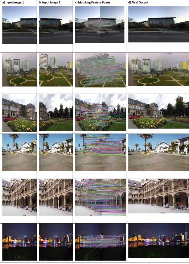
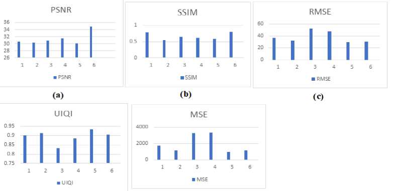
6.    Experimental Results

In this paper, image stitching based on invariant features is proposed. The main step in image stitching is calibration, image registration and blending. For image registration, SIFT algorithm is applied. The feature descriptors are matched using BF matcher with KNN algorithm. Outliers are eliminated using RANSAC. Image blending is performed to remove the visible seam.

In SIFT algorithm, initially scale space of each input image are constructed. From the scale space Difference of Gaussian (DoG) is calculated. DoG function is used to obtain the scale-space extrema points. Scale space peak selection aims to find out the potential location of the key points. The locations of the detected key points are identified accurately in the next step. Scale space construction is required to make the feature detector invariant to the scaling operation. Feature points located at edges and low contras features are discarded. To attain rotation invariance, different orientations of feature points are considered and dominant orientation is finally selected as the orientation of that particular feature point. The last step in SIFT in feature descriptor creation. The magnitude and orientation of each key points are calculated to create the feature descriptor. Feature descriptor is a vector and its length is 128. To identify the overlapping area, feature points of each input images are compared with each other using Brute Force (BF) matcher with KNN algorithm. RANSAC algorithm is used for eliminating the remaining outliers in the feature points. Input images are aligned together by applying perspective warping transformation. The presence of distortions is removed by warping operation. Finally visible seams are removed by using alpha blending.

The proposed algorithm is implemented on six set of different images on UDIS-Data set. It is a large collection of real-world images that can be used for stitching and registration. It includes several overlap rates, levels of parallax, and scene variations including indoor, outdoor, night, dark, snow, and zooming. We took images from different background like images taken in light, dark and images with different ranges overlap and parallax. The size of the images taken from this data set is 512× 512-pixel size.

The result obtained on the above data set using the proposed algorithm is shown in Fig. 4. The first column in the Fig. 4 represents the original input images, the second column is the corresponding image that is to be stitched with the first image. Corresponding feature points in two input images are shown in third column. The final stitched image is given in fourth column.

From the Fig. 4 it is clear that illumination difference is eliminated in the final image and there is no visible seam across the stitched image.

The feature detectors are compared based on the number of detected features and matched features using six different sets of images. The overall stitching performance is evaluated based on different evaluation metrics such as PSNR, SSIM, RMSE, MSE and UIQI. The performance evaluation result is shown in Table 1.

Table 1. Performance Evaluation of Image stitching

Input Image Set	PSNR (dB)	SSIM	RMSE	MSE	UIQI
1	30.68	0.7808	37.43	1717.78	0.9005
2	30.34	0.5521	32.38	1139.30	0.9140
3	30.89	0.6527	52.75	3291.08	0.8317
4	31.56	0.6209	47.72	3334.72	0.8866
5	30.15	0.5896	30.53	971.343	0.9326
6	34.84	0.7970	31.05	1177.440	0.9059

From the Table 1, it is evident that the PSNR value is high in image 6. Typical PSNR values in image reconstruction are between 30dB and 50 dB, assuming an image having 8-bit depth. The highest value gives the better result. The value of SSIM ranges from 0 to 1, with 1 denoting a very good match between the reconstructed image and that of the original image. Here the SSIM value is also high for image 6 and 1 as compared to other five image pairs. The high value of PSNR and SSIM indicates that the good quality of the stitched image. So, image set 6 have better quality based on PSNR and SSIM compared to image 1. RMSE and MSE is low for image 5 and image 6. Among these two images 5 has less error. The low value of RMSE and MSE indicates less stitching error. UIQI is another evaluation method; its high value denotes good quality in the output. UIQI is high for image 5. In total, comparing all parameters and physical appearance of the stitched image, out of 6 images image 5 has high quality in stitching.

The graphical representation of the performance evaluation is shown in Fig.5. By evaluating the visual quality of the stitched image, the proposed method’s qualitative performance is assessed. No seam was present in the stitched image. It indicated the efficiency of stitching. If variation in rotation is too high, blank region will be occupied in some portions of the image after warping. This can be eliminated by applying image in painting algorithms, which automatically fill the region by applying the pixel values in the neighbor region.

Fig. 4. a) Input Image 1 b) Input Image 2 c) Matching Feature Points d) Final Output

(Й)

(е)

Fig. 5. Graphical representation of performance evaluation. (a)PSNR, (b)SSIM, (c)RMSE, (d)UIQI, (e)MSE

7.    Conclusion

In this paper, we proposed an invariant feature extraction-based method for stitching images. The proposed method creates panoramic image without visible seams. For feature detection, the Scale Invariant Feature Transform (SIFT) is used. These features are rotation and scale invariant additionally, somewhat invariant to variations in illumination and 3D camera perspective. Feature points are matched by using BF matcher with KNN algorithms. Outliers in the feature points are removed by using RANSAC. This increases the accuracy of the set of matching feature points. Proposed method is implemented on UDIS data set. Six set of different images are used for the experiment. Presence of distortions in the images are removed in the alignment operation through perspective warping. The visible seams across the stitch are successfully eliminated by alpha blending method. the proposed method perfectly stitches multiple images of varying scale and orientation and produced seamless panoramic image. Using evaluation criteria such as PSNR, SSIM, RMSE, UIQI, and MSE, the overall performance of the proposed stitching is evaluated. The proposed seamless image stitching algorithm yields a good result. Comparing with the state-of-the-art methods discussed in literature survey, the proposed image stitching method has better performance. The limitation of SIFT in image stitching is, if the number of images is too large, it takes more time for feature detection. Comparing SIFT with SURF, ORB and FAST algorithm, in FAST the performance will reduce if high noise levels are present whereas SIFT is robust to noise. SURF has poor performance under color and illumination changes and it is not stable to rotation. In the case of ORB scale change is not considered. Deep learning based homography estimation can be developed as a future enhancement of this problem. Another direction for future work is collaborating image inpainting techniques to fill the blank area in the stitched image.