Segmentation of the herniated intervertebral discs

Published Online June 2018 in MECS DOI: 10.5815/ijigsp.2018.06.04

• I.    Introduction

  Human spine provides the main support to the body that helps us to stand erect, bend, twist and also helps in providing a protective shell to the spinal cord. It consists of bones, cartilage, ligaments and muscles (Schmorl, Georg, 1959). If any of the parts of the spine are distressed by strain or injury or any disease, it can cause severe pain. Back pain is considered to be the second highest health issue after common cold and is regarded as the second most common reason why patients visit doctors’ clinic in USA(Alomari, Corso, Chaudhary,

  2011). It is also considered as one of the major prominent chronic diseases that causes lot of disruption in peoples’ lives (Alawneh, Al-dwiekat, Alsmirat, Al-Ayyoub, 2015). The human spine is made up of 33 individual bones, called as vertebrae, interlocked with each other. These vertebrae are divided into unique regions; 24 from the top are cervical, thoracic and lumbar, which are movable, the rest 9 are sacrum and coccyx which are fused as shown in the fig 1a. Every vertebra in the spine is isolated and padded by an intervertebral disc, shielding the bones from rubbing together. The intervertebral discs are comprised of an adaptable ring of collagen strands called the annulus fibrosus which is loaded with delicate gel like substance called nucleus pulposus. The intervertebral discs are actually cartilaginous in nature and are shown in the fig 1b (Michopoulou et al., 2009).

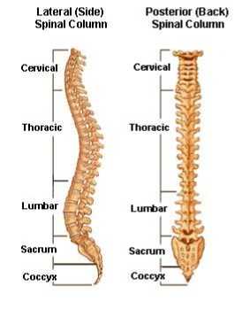
Fig.1a. Showing different parts of the spine.

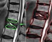
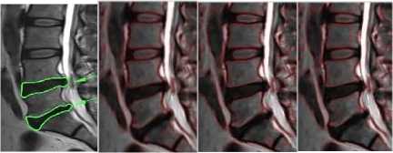
Aging, trauma, genetic disorders, nutritional disorders usually result in the degeneration of the intervertebral discs (Michopoulou et al., 2009). And among all the disc degenerative disorders’ disc herniation is one of the major disorders resulting in the major causes of back pain (Koh et al., 2010). In disc herniation the outer ring, i.e. the annulus fibrosus ruptures resulting in the leakage of the central gel-like material, the nucleus pulposus as shown in the Fig 2a and Fig 2b. In such a disorder, the gel like material puts enough pressure on the spinal nerves and causes swelling or what we call as inflammation of the nerves that are around, which results in severe back pain, radiating pain, and muscle spasm (Milette, Pierre, 2000).

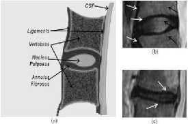
Fig.1b. Chematic of a midsagittal cut of the human spine demonstrating the major anatomical components, as well as (b) normal and (c) degenerated intervertebral disc (10. Michopoulou, et al., 2009).

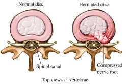
Fig.2a. Showing annulus fibrosus tear resulting in nucleus pulposus leakage and nerve compression (©Baker Chiropractic).

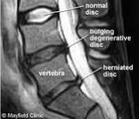
Fig.2b. MR Image showing the difference between normal and a herniated disc. There is a difference in the intensity of the signal of nucleus pulposus of normal disc and that of the nucleus pulposus of the herniated disc.

The rest of the paper is presented as: section II discusses literature review. Section III describes the methodology and its implementation. In section IV details of the clinical data set used is provided and in section V experimental results are given and their details are discussed in section VI and the conclusion of the work done is discussed in section VII.

• II.    Related Work

  A very limited work has been done on the segmentation of the herniated discs and is illustrated in the table I. The accuracy and the level of the automaticity of the disc herniation diagnosis done previously are also mentioned in the table. Tsai et al (2004) adopted a method in which geometrical features like shape, size and location were used to diagnose herniated discs 3D MRI and CT transverse sections. In another work by Koh, Jaehan, Vipin, Gurmeet (2010) diagnosis of disc herniation is done based on classifiers and features generated from spine MR images. Three different classifiers have been used: support vector machine (SVM) classifier, a perceptron classifier, and a least mean square (LMS) classifier. 68 clinical cases were studied and gave 97% accuracy. Alomari, Corso, Chaudhary, Dhillon, (2014) used active shape model and an active contour model to help in the segmentation and feature extraction for the detection of lumbar spine disc herniation. Bayesian classifier and a Gibbs based distribution with shape potentials has also been used. Initially disc localization has been done using two level probabilistic model, earlier proposed by Corso, J. J., Raja, Chaudhary,

Table I. Illustrating the accuracy and level of automaticity of the previous work on herniation diagnosis

S.NO	PAPER	SCANS	SCAN TYPE	ACCURA CY [%]	AUTOMATICITY? (slice, detection, segmentation)
1.	Tsai et al [2004]	16	Axial MRI or CT	Information not available	Fully manual
2.	Koh et al [2010]	68	Sagittal T2	97	Fully manual
3.	Koh et al [2012]	70	Sagittal T2	99	Fully manual
4.	Ghosh   et   al [2011b]	35	Sagittal T2-SPIR	98.3	Mid scan, axial interaction, automatic segmentation
5.	Ghosh   et   al [2011a]	35	Sagittal T2-SPIR	94.9	Mid scan, axial interaction, automatic segmentation
6.	Alomari  et  al [2010a]	33	Sagittal T2-SPIR	91	Manual selection, information not available, information not available
7.	Alomari  et  al [2011b]	65	Sagittal T2-SPIR	92.5	All slices, information not available, automatic segmentation
8.	Alomari  et  al [2013]	65	Sagittal T1- T2	93.9	Manual selection, information not available, automatic segmentation
9.	Khaled Alawneh et al [2015]	32	Axial MRI	100	Information not available

(2008). Alawneh, Al-dwiekat, Alsmirat, Al-Ayyoub, (2015) proposed a computer aided diagnosis system for lumbar disc hernia and have tried to extract the ROI by adaptive thresholding and determining the ROI horizontally, which means top-down MRI scans were used instead of the sagittal view, with a fixed displacement before and after the closest point to the spine. Later ROI was enhanced by CLAHE, followed by feature extraction by skeletonization. Michopoulon et al., (2009) used intensity based classifier and have implemented three different fuzzy C-means algorithms for atlas based disc segmentation. The same algorithm was also used for classifying a disc as a normal or an abnormal one.

As per the survey the techniques implemented in this work, which are distance regularized level set segmentation and morphologically preprocessed watershed segmentation, have not been implemented for the diagnosis of the disc hernia before. Level set segmentation is the preferred segmentation algorithm as far as the contour evolution of complex topologies is considered and is able to deal with the topological changes in a better way (Qin, Zhang, 2009). There is another advantage and is that, there is no need to parameterize the points on a contour; computations are done on a fixed Cartesian grid (Xu, C., Prince, J. L., 1998). Distance regularized level set evolution has been implemented which eliminates the requirement of reinitialization resulting in reducing the computation time and induced numerical errors. As stated by (Chevrefils,

Cheriet, Aubin, Grimard, 2009) watershed segmentation technique can handle wide variety of shapes and topologies. Watershed segmentation works in poor contrast as well and hence post processing requirement is eliminated, such as joining of contours. The methodology and the implementation of both these methods are discussed in depth in the next section.

• III.    Methodology and Implementation

  Segmentation of medical images is a very crucial step in a multiple of medical applications (Bouzid-Daho et al., (2018). Kalaiselvi, et al., (2017). Lakshmi, et al., (2017)). There are number of automatic and semi-automatic segmentation methods, (Pan, et al., (2013), Ruiz-España, et al., (2015) Erdil, et al., (2013), Chevrefils, et al., (2007). ) and amongst them none of the methods is considered as the perfect one because of the different types of unknown noise present, poor image contrast, weal boundaries, complicated structures of the human body. Also the intensity distribution in the medical images is very complex (Balafar, et al., (2008). The methods implemented in this paper are discussed below.

• A.    Level set segmentation

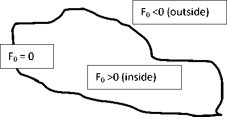
  Level set method has been initially put forward by Osher, S., Sethian, J. A., (1988). A numerical solution was proposed for processing topological changes of the contours. Level set method has been extensively used in image processing and especially in the field of image segmentation and multiple level set based segmentation algorithms have developed (Pan et al., 2013)( Ferhat et al., 2014) (Shen, Yu, Liu, Chen, 2010)( Huang, Jiang, 2009). What actually happens in level set method is that, if we have a given image I 0 and F 0 is its level set function which is used to interpret the aimed contour C. Each pixel of the image I ₀ will have a corresponding level set function value (F ₀ ). We define the contour as the region where level set function is zero, that implies, F ₀ = 0 and the region inside the contour is the region where level set

function is greater than zero and the region outside the contour is less than zero. So with the change in the value of the level set function, there will be corresponding change in the region that is outside the contour and inside the contour and with result the boundary which is F ₀ = 0 will be different and hence the contour will evolve.

In our approach we have used the concept of the distance regularization (Li et al., 2010) in which there is a concept of an external energy which drives the motion of the zero level set towards the desired location. In this approach the gradient magnitude of the level set function is forced to one of its minimum points by a term of potential function and hence maintains a desired shape of the level set function.

In practice an observed image can be expressed as

I = BI ac + П                   (1)

Where I _ac is the actual image, B is the Bias field which can be a result of intensity inhomogeneity in MR images, n is the additive noise and the term I _ac is an inherent physical property of the imaged objects which has N distinct constant values C 1, …, C N in disjoint regions Ω 1 ,…, Ω N , that means

Q = u f=1 Q i Q i П Q j = 0 i* j         (2)

Also the shading image what we call as the bias field is varying very slowly which means ‘B’ can be taken as a constant. In our approach standard K-means clustering (Kanungo et al., 2002) is used to classify the local intensities as because of the intensity inhomogeneity it is very difficult to segment the overlapping regions based on the pixel intensities.

The K-means clustering can be defined in a continuous form as

E y = Z zU J^K^ — x)|7⁽x) - B(y)c_z|²dx    (3)

where K(y-x) is a Gaussian function. Smaller the value of E y better the classification, therefore, it is required to minimize E y for all values of y in Ω and can be achieved by minimizing the integral of E y with respect to y and hence energy is defined as E = J E_ydy, that means,

E = J(E /=i J^ =1 ^(y — x)|7⁽x) — S⁽y)C i ^|2dx) dy  (4)

During the level set evolution C i and B are updated by minimizing the energy function E(F 0 , C, B)

E(F o ,C,B) = JZ i=o e i (x)M i (F o (x))dx

Where Mi(F0(x)) is the membership function which represents the phase indicator for the regions and the level set function given by F0 and ei(x) is defined as ei(x) = J K(y — x)|7(x) — S(y)Ci|2dy (6)

The energy minimization with respect to the level set function F0 is given as aF0 _ aSF at = at

where SF represents the speed function that controls the evolving level set.

SF(F0, C, B) = E + ^5(F o )div() + y5(F₀)|VF₀|  (8)

|VF0| where 5(F0) represents the dirac function which is the derivation of Heaviside function and ^ , у are the regularizing constants.

As far as the implementation in concerned, it is very straightforward. Initially scale parameters are defined. For example, sigma ‘a’, which is the standard deviation of the Gaussian function of K-means clustering. The effect of the a, is being discussed in detail in the section VI of the paper. The other parameters like, time step, Vt has been put equal to 0.1, regularization parameter ^ is set equal to 1.0 and у is usually set to 0.001 * 255 2 as a default value for most of the digital images with intensity range in [0.255]. Then level set function is initialized. After initialization Gaussian kernel is defined as a w*w mask, where w is the smallest odd number, w > 4 * a + 1. Once iteration of the level set function is started, each iteration is modeled using Gaussian probability distribution. Then the zero level contour is updated. The iteration processes is terminated once the final contour is obtained by the saturation of the energy of the object/background, or the predefined iteration limit is acquired, if not then the iteration of the level set function is again started.

• B.    Watershed segmentation :

Another technique, that is, watershed segmentation is implemented along with some morphological preprocessing. In the preprocessing steps image normalization is done to reduce the effect of variation in the input images. Two common methods are:

• 1.    Contrast stretching

• 2.    Histogram equalization

The details of the data set on which these algorithms have been implemented are provided in the next section.

• IV.    Clinical Data Description

  The data set used for the evaluation has MR images of 69 cases, ranging from age group of 16 to 78 years. The data set has been acquired from MEDICARE, a private diagnostic center at Srinagar, India. The sagittal, T2-weighted, MR images in DICOM format, provided by MEDICARE, have matrix resolution mostly of 240*240 and 256*205, slice thickness ranging from 1.7 mm to 6 mm and slice gap ranging from 20 to 300 percent, TR ranging from 3.3 milliseconds to 7.8 milliseconds and TE ranging from 1.27 milliseconds to 3.69 milliseconds and flip angle ranging from 8 degrees to 20 degrees. The simulation platform used is MATLAB 2010. A total of 12000 scans are compared with the golden standard, i.e., the manually segmented images, done by the doctors at the Radiology Department of a medical institute in Kashmir, India.

• V.    Experimental Results

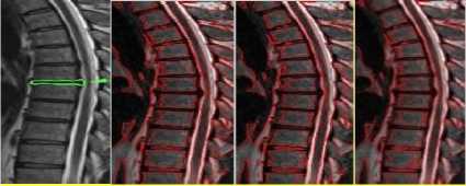
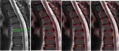
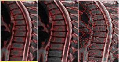
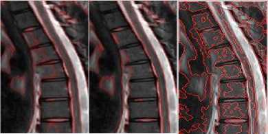
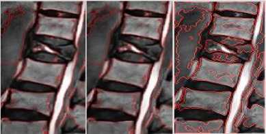
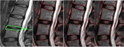
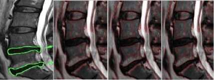
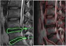
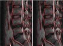
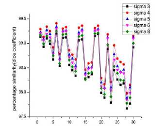
To analyze visually the results, 2D images corresponding to the segmentation process in thoracic and lumbar regions are shown in the fig 3 and fig 4 below, respectively. Also the effect of the c, i.e., the standard deviation of the Gaussian kernel used in the level set segmentation is shown in the figures.

The results obtained from the Automatic segmentation methods are compared with the golden standard. The comparison is performed using the DICE and JACCARD coefficients (Ruiz-España, Díaz-Parra, Arana, Moratal, 2015) (Michopoulou, et al., 2009) (Huang, Chu, Lai, Novak, 2009) and is given in Table II.

DICE coefficient is defined as

DICE =

where GS is the golden standard and SegIm is the computed segmentation volume in voxels.

JACCARD coefficient is given by

JACCARD =

|GSnSe.g/m|

MARKED   SIGMA 3    SIGMA 4    SIGMA 5

SIGMA 6     SIGMA 8       WS

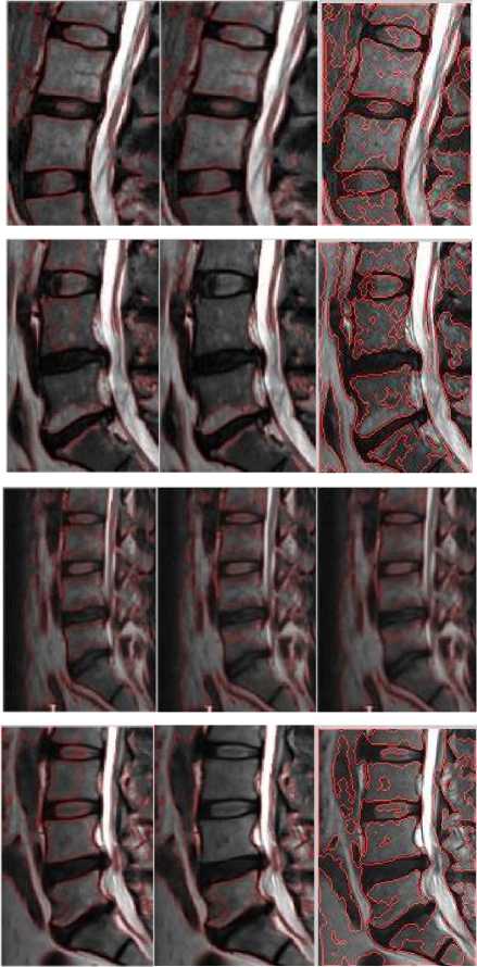
Fig.3b. Column 1, 2: level set segmented image of the thoracic regions at different values of □, column 3: watershed segmented image.

SIGMA 6      SIGMA 8        WS

Fig.4b. Column 1, 2: level set segmented image of the thoracic regions at different values of o, column 3: watershed segmented image

MARKED SIGMA 3   SIGMA 4 SIGMA 5

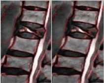
Fig.4a. Column 1: manually segmented image, column 2, 3, 4: level set segmented image of the thoracic regions at different values of o.

patients without disc abnormality

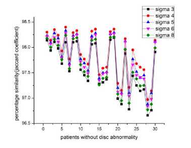
Fig.5a. Effect of sigma-patients without any abnormality.

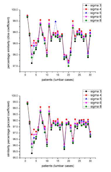
Fig.5b. Effect of sigma-patients having disc hernia in lumbar region.

These experimental results are discussed in the next section.

• VI.    Discussion

In sagittal, T2 weighted MR images a normal intervertebral disc appears as a bright spot at the center representing nucleus pulposus (which has 85% - 90% water content under normal conditions) surrounded by a dark ring which represents annulus fibrosus. In disc herniation because of the disc degeneration there is a chemical change (reduced water content) in the composition of the nucleus pulposus resulting in a localized displacement of the disc material. As far as the visual inspection is considered we can observe in the fig

• 3 and fig 4 that the bright spot is missing in the degenerated discs, that is the nucleus pulposus is missing and the darker ring, which is the annulus fibrosus, is ruptured and is protruded outwards, stressing the spinal canal resulting in the pain and discomfort. In some cases whole nucleus pulposus is not missing, it is either deformed or a portion is missing indicating initiation of the disc hernia. In level set segmentation the results are better at с = 4, i.e., when the standard deviation of the Gaussian function of the K means clustering is equal to 4, the moment we increase the value of the с the results get deteriorated. As can be seen from the figures 5a, 5b and 5c, the highest peaks corresponds to с =4. Fig 5 illustrates the percentage similarity when the segmented images are compared with the golden standard at different values of с. Fig 5a, 5b and 5c illustrates percentage similarity of the patients without any abnormality, with abnormality in the lumbar region and the last one with abnormality in the thoracic region, respectively. . From the table II it is evident that both DICE and JACCARD coefficients support the comparison done on the visual inspection basis. It can be noted from the table II that both the similarity indices have lesser values for the thoracic region of the spine as compared to that of the lumbar region irrespective of which algorithm we have used. It can be because of the closeness of the spine in the thoracic region to the corresponding ribs (Ruiz-España, Díaz-Parra, Arana, Moratal, 2015). Another observation is that the jaccard similarity index has lesser values than corresponding dice similarity index. Jaccard index is calculated by the ratio of the intersection of the two images by their union while as the dice index is calculated by the ratio of the area of mutual overlap to the sum of the areas of the golden standard and the segmented image. Third observation is that watershed segmentation is giving better dice and jaccard coefficients as compared to the level set segmentation technique. Level set segmentation technique requires lot of fine tuning of parameters in order to obtain the desired results and also is dependent on the initial conditions while as watershed segmentation used is a morphologically preprocessed algorithm that works on the prior knowledge of the shape of the object. It can be easily noted that our techniques provide significantly improved segmentation accuracy in comparison with the disc herniation diagnosis done previously by the different authors as illustrated in the table I.

Both these algorithms are fast, unsupervised, and do produce closed contours. Level set segmentation algorithm implemented is relatively slower as compared to the watershed segmentation algorithm (Table III) but watershed segmentation has an inherent disadvantage of over-segmentation which can hinder the results.

In table III corresponding manual and automatic segmentation times are given.

Table III. Manual and Automatic segmentation times

SEGMENTATION METHOD	MANUAL INTERACTION TIME (s)	PROCESSING TIME (s)
Level          Set Segmentation	10	18
Watershed Segmentation	10	2
Inter-observer	150

Table II. Illustration of the automatic segmentation performances.

LEVEL SET SEGMENTATION a = 3
AVERAGE (MEAN ± SD)	DICE COEFFICIENT		JACCARD COEFFICIENT
	THORACIC [%]	LUMBAR [%]	THORACIC [%]	LUMBAR [%]
	98.513±0.541	98.578±0.524	96.87±0.93	97.33±0.78
MINIMUM	97.69	97.5	95.47	95.36
MAXIMUM	99.12	99.67	98.15	99.34
LEVEL SET SEGMENTATION a = 4
AVERAGE (MEAN ± SD)	DICE COEFFICIENT		JACCARD COEFFICIENT
	THORACIC [%]	LUMBAR [%]	THORACIC [%]	LUMBAR [%]
	98.98±0.433	98.80±0.4832	97.5644±0.81	97.769±0.73
MINIMUM	98.13	97.75	96.32	96.10
MAXIMUM	99.49	99.75	98.72	99.49
LEVEL SET SEGMENTATION a =5
AVERAGE (MEAN ± SD)	DICE COEFFICIENT		JACCARD COEFFICIENT
	THORACIC [%]	LUMBAR [%]	THORACIC [%]	LUMBAR [%]
	98.72±0.50	98.71±0.51	97.22±0.82	97.55±0.78
MINIMUM	97.92	97.65	95.93	95.92
MAXIMUM	99.35	99.71	98.32	98.78
LEVEL SET SEGMENTATION a =6
AVERAGE (MEAN ± SD)	DICE COEFFICIENT		JACCARD COEFFICIENT
	THORACIC [%]	LUMBAR [%]	THORACIC [%]	LUMBAR [%]
	98.76±0.4747	98.71±0.48	97.21±0.84	97.58±0.76
MINIMUM	98.09	97.69	96.26	96.06
MAXIMUM	99.29	99.72	98.48	99.45
LEVEL SET SEGMENTATION a =8
AVERAGE (MEAN ± SD)	DICE COEFFICIENT		JACCARD COEFFICIENT
	THORACIC [%]	LUMBAR [%]	THORACIC [%]	LUMBAR [%]
	98.61±0.50	98.62±0.51	96.99±0.88	97.42±0.81
MINIMUM	97.83	97.51	95.76	95.81
MAXIMUM	99.21	99.70	98.24	99.41
WATERSHED SEGMENTATION
AVERAGE (MEAN ± SD)	DICE COEFFICIENT		JACCARD COEFFICIENT
	THORACIC [%]	LUMBAR [%]	THORACIC [%]	LUMBAR [%]
	99.22±0.226	99.29±0.31	98.45±0.45	98.6±0.61
MINIMUM	98.86	98.67	97.74	97.37
MAXIMUM	99.44	99.84	98.89	99.68

• VII.    Conclusion

Disc hernia is a major spine abnormality these days which results in persistent back pain and is considered to be a major reason why patients visit radiologist clinic these days. As per the researchers and projectionists there will be severe inadequacy of the radiologists in near future as the demand of radiologists is drastically increasing day by day, and is much greater than the patients (Sreeji, Vineetha, Beevi, Nasseena, 2013). Since picture archiving and communication system (PACS) has helped a lot in the retrieval and visualization part (Erdt, Steger, Sakas, 2012), so a Computer Aided Diagnosis System (CAD), which can help in generating diagnostic results from clinical MRI, CT scans or even X-rays, would reduce the burden on radiologists and can help in on time diagnosis as well in surgical intervention whenever needed. This attention has inspired the authors of the manuscript to make an attempt that would help in developing a CAD system for the diagnosis of herniated intervertebral discs. Segmentation is considered as a very essential analysis function as for as CAD system is considered. Segmentation is all about segregation of structures of interest either from the background or from each other. In medical image processing, image segmentation is a very important analysis phase for characterization of different components, such as for analyzing different anatomical structures, different tissue types, or different pathological regions. Image segmentation can also be helpful in image guided surgeries, tumor radiotherapies or in evaluation of therapies. Medical images mostly contain strong noise and inhomogeneity as a result segmentation is abit difficult task. In this paper we have implemented two automatic segmentation techniques for lumbar disc herniation diagnosis, and have compared the results with the golden standard. One of the segmentation algorithms is variational level set segmentation and another one is watershed segmentation technique. Implementing both these techniques can help a radiologist in quick and accurate computer aided disc herniation diagnosis and surgical intervention, whenever needed. In level set segmentation technique effect of the change in the standard deviation of the Gaussian function of K means clustering is also seen. With the increase in the values of the standard deviation segmentation results are getting deteriorated. Watershed segmentation technique is giving better accuracy both in the thoracic and lumbar parts of the spine as compared to the level set segmentation but has a disadvantage of over-segmentation. Future work will focus on the classification of the herniated disc and the possibility of using other modalities for diagnosis of herniated discs.

This work is an extended version of our previous work (Mir, A. H, 2014).

Acknowledgment

The authors wish to thank the Department of Radiology of SKIMS, Kashmir, especially Dr. Azhar for helping in evaluation.