Seismic refraction modeling using finite difference method and its implications in the understanding of the first arrivals

Introduction                                analyzing various problems mainly in the exploration of hydrocarbons. Their algo-

As described in Dobrin (1976), the seis-  rithms have been improved in terms of the mic modeling has been an important tool for numerical approximation and propagation in

the elastic mediums (Sayers, 2009). According to Bridle (2016), and due to the inclusion of geophysical methods in the determination of exploration geotechnical data, the seismic modeling was taken to study the behavior of waves on different geometries and acoustic contrast between layers (Budhu, 2010). For example, such as the contact between soil and residual colluvial deposits, where the acoustic impedance is low, and the contact between the colluvial deposits and bedrock, where the impedances high (Redpath, 1973).

In this work, we study the propagation of head waves in an elastic medium over a contact between unconsolidated sediments and bedrock, which enables to see the changes in the first arrivals of the P wave on the surface, showing significant changes in the traveltime curves in the areas with tilt refractors (Lankston, 1988). Traditionally, the modeling of the seismic refraction focuses in calculating the first arrival time (FAT), which is performed using mainly the time-term method (TTM). An example of this method is shown in (Iwasaki, 2002) and (Berry et al, 1966). In this work, to study the first arrivals picking, the method of finite differences (FDM) was used, because it allows one to analyze the times (FAT) and the record of the wave propagation for each geophone. Finally, a comparison using linear fitting, coefficient of determination, and residual mean square between the results obtained by FDM and TTM modeling was made.

Methodology

The modeling by time-term method (TTM) was conducted using the module of the Plotrefra (SEISIMAGER), which includes the capability of creating a custom velocity model for forward modeling purposes. The first arrival time was calculated by time-term method, according to (Bath, 1978). This technique is a linear least-squares approach to determine the best discrete-layer solution to the data. The math behind this technique is comparatively simple. A two layers single receiver-source model is showed in Fig. 1 with the next configuration;

V 1 and V 2 are the velocities for the layer 1 and 2 respectively; i c is the critical angle; Z 1 and Z 2 are the perpendicular depth measure from source and receiver position respectively. In this case, the time ( t ) is calculated as shown in the following equation:

t = cz_l + cz₂ + xS₂          (1)

where Sj = 1/ v, S2 = 1/ v2 ,and c = 2S 1 cos(ic), Si, S2 -slowness in layer 1 and 2 respectively, c - substitution constrain slowness-dependent, x -distance from source to receiver.

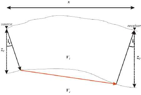
Fig. 1. Two layers scheme to explain the calculation of the trajectory and time by TTM method. Modified from (Iwasaki, 2002)

Generalizing the equation (1) for a model with multiple layers, tj=^ cjkzk + xjS 2          (2)

k = 1

we get in a matrix form:

' c11 c12 • c1n x 3 ' z 1 3 (' 1 3 C 21 c22 • c2n x2 z 2 t2 C 31 c32 • c3n x3 -■3 = t3 C 41 c42 • c4n x4 • t4 • • • • • n • l cm 1 c m2 • c mn x m 7 [ S 2 7 1 tm 7 where number of travel times j = 1..m, and number of receivers k = 1..n (depths to be calculated). In this case, it is possible to solve the matrix for Z1…Zn and S2.

The first arrival time calculation using the finite difference method (FDM) was performed using the free software package SeismicUnix (program SUFDMOD2), which works on the Linux operating system (in this work, Fedora 20). This program uses finite-difference method (Stockwell, 1999) to solve the 2D acoustic wave equation:

д ² ф ( x , z , t )      2         2

----—----= v (x, z)V ф(x, z, t),   (3) д t where v(x,z) is the velocity in the acoustic media.

The Laplacian operator can be approximated with central difference operators. Where the velocity, spatial sampling rate, and grid spacing are in consistent units.

n+1         n       n-1        n           nn v2лn   фj  - 2ф + фj   , фj+1 - 2ф + фj-1

V ф ~     Ax2           Az2w

The time derivative is calculated by a second order finite difference scheme:

д ² ф (t ) ~ ф (t + A t ) - 2 ф ( t ) + ф ( t - A t )

Cl'                  At2

Finally, each finite difference scheme has a stability condition (Slawinski et al, 1999). The stability condition for the second order scheme used by SUFMOD2 is shown in the equation 6. This program does not require the grid spacing to be equal in the horizontal and vertical directions. Figure 2 describes the general flow diagram with the list of processes required in SUFDMOD2 for the generation of synthetic seismic records. To create models with complex geometry, we recommend using the package TRIMODEL, which calculates a triangulated velocity model of subsurface. Subsequently, this model is made uniform by using the program TRI2UNI. In this work, three variants of the same model, which differ only in the grid spacing, were studied. In the Table 1 ∆ z and ∆ x are the spatial interval in the z-axis and x-axis respectively, and nx and nz are the sample numbers in the z-axis and x-axis respectively.

v m^ax^{A t} < I¹ (6) A x П

V max - maximum velocity in the model (m/s);

∆ t - time interval in seconds;

∆ x - spatial interval in the x-axis (meters).

Table 1 . Grid spacing parameters

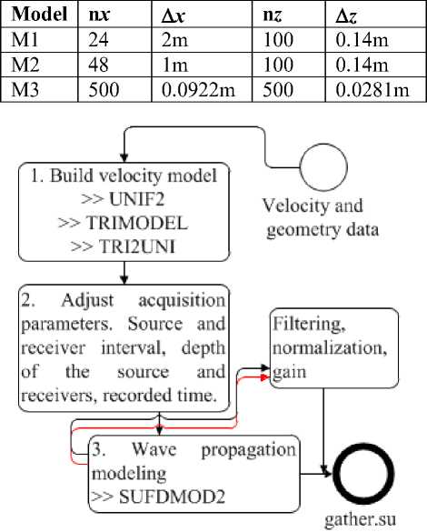
Fig. 2. A general processing flow diagram of using SUFDMOD2 program in SeismicUnix

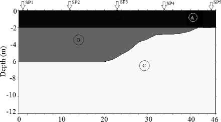
We used for both modeling methods the general model shown in Fig. 3 with the area of thickness of 2 m simulating a geometry of the completely flat refractor. The zone B (1250 m/s) has a variable thickness 0 - 4 m that corresponds to a refractor with complex geometry simulating the advanced processes of weathering on the bedrock indicated in the general model by the area C. We used a sequence of five shot-points with different location. Table 2 shows the position of each shot.

Table 2 . Shot points location

Shot point	Location
SP1	1 m
SP2	12 m
SP3	23 m
SP4	34 m
SP5	45 m

Distance (m)

Table 3 . Computing parameters during the model generation by the SUFDMOD2 program for different grid spacing

Model	No. ofitera-tions	CPU time	Stable △ t(s)
M1	3450	1.101 s	2.898e-05
M2	3751	1.745 s	2.665e-05
M3	18761	436.17s	5.338e-06

Fig. 3. General model. (A) Colluvial zone Vp1=300m/s; (B) residual soil zone Vp2=1250m/s with flat refractor at z=-6m and complex refractor at x= (20, 42) m; (C) bedrock zone Vp3=2500m/s

Distance (m)

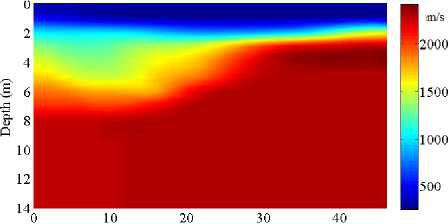
Fig. 4. Uniformly sampled velocity model of layered medium (M3) in binary format used for SUFDMOD2 program

The uniform models (Fig. 4) were built using linear interpolation of the data obtained by seismic tomography. SeismicUnix creates different models using the program UNI2, which generates a 2-D uniformly sampled velocity profile from a layered model. In each layer, velocity is a linear function of position.

Results

The modeling with finite differences for the velocity model with 3 different grid spacing (Table 1) produced a variation in the optimization of stable ∆ t (6) and the number of iterations (Table 3).

A seismogram with the traces corresponding to the registration of the P wave to geophone spread was obtained for each model settings, which differ in values n x (number of samples in x-axis) and n z (number of depth-samples) .

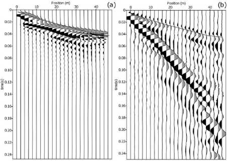
It was found that the variation in the number of geophones used for seismic acqui- sition has a significant impact on the quality of registration of seismic events. In the seismogram with nx=24 (Fig. 5), the first break of refracted wave is reliably identified, but the accurate arrival time of the direct wave close to position of the source is difficult to define. Using nx=48 (Fig.6), we are able to improve the sampling of the waves between 0.04 and 0.05 seconds, and only seismogram obtained with nx=500 (Fig. 7) shows clearly the head waves 1 and 2, and direct wave.

The results obtained using TTM and FDM methods are illustrated in Fig. 8. The time of arrival of the P wave on the same model using n x = 24 was calculated with each method. In Fig. 8A, the comparison between the travel-time curves shows a high dispersion of the data for time less than 0.015 s. For times exceeding 0.015 s (first refraction time in Fig. 8C), the evidenced changes in the slopes of the curve corresponding to the different layers of the subsoil are clearly recognized. The highest difference (FD – TTM) about 0.008 s (Fig. 8B) corresponds to the direct wave. To analyze the dispersion of the results, we performed a linear fit between them shown in Fig. 8C.

This curve was divided into two zones (high correlation zone and low correlation zone). The value of calculated coefficient of determination was determined as 0.956866 and the straight fit equation was defined as timeRT =1.07871478* timeFD - 0.00284832, where timeRT and timeFD are the times calculated from TTM and FDM data respectively.

Analysis of the seismic survey data

A seismic refraction survey in Barranca-bermeja (Colombia) was developed with the aim to identify changes in the subsurface and define the depths and types of soils.

The seismic acquisition was performed using a seismograph ES-3000 with 24 vertical 14 Hz geophones separated 2 meters. The total length was 46 meters. The result of the seismic processing is shown in Fig. 9. The results of seismic tomography processing correlate with the data of the geotechnical survey.

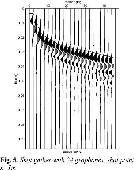
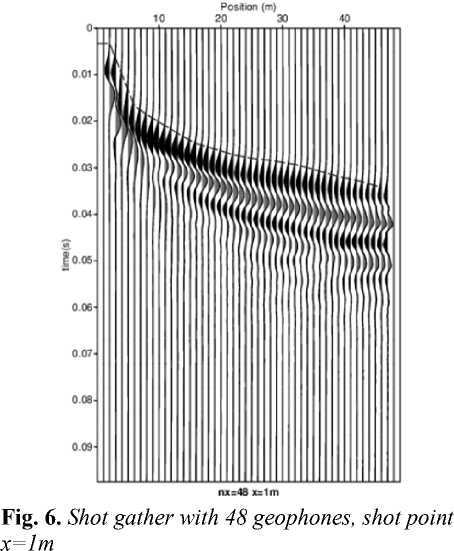
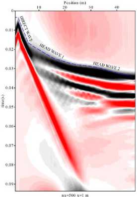
Fig. 7. Shot gather with 500 geophones, shot point x=1m

For optimization the temporal parameters in future acquisition surveys over the same area, we performed a seismic modeling using FDM. Additionally, the modeling allowed us to know the validity of the obtained results by comparing the synthesized traces with the survey traces (Fig. 10).

The events associated with the refraction waves were found between 0 and 0.05 seconds. The seismic survey should decrease the maximum time of the acquisition but increasing, on other hand, the detail of the head waves to improve the process of first arrivals picking.

The arrival times obtained in the seismic record x=0m using FDM and real data, procurement of field (RD) are shown in Fig. 11.

The slope preserves the general trend, but the data differ in terms of lap times. In blue curve shows the difference between two times. The maximum difference is 0.011 seconds.

Conclusions

Modeling using the finite difference method showed precision in the calculation of the first arrival time of P-wave, which was verified using statistical correlations among the times calculated by the TTM method and the times obtained from the seismogram (first arrival time picking using the FDM method).

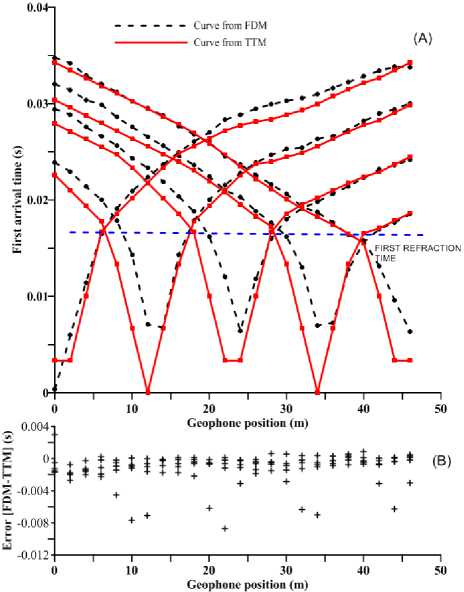
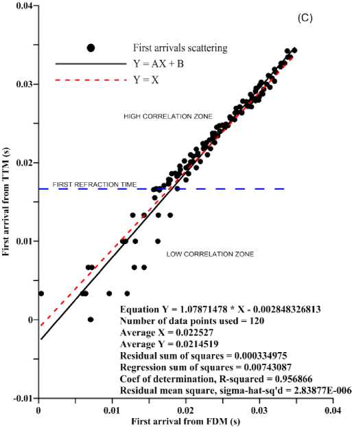
Fig. 8. First arrival times obtained using FDM and TTM. (A) travel time curves, (B) time difference between methods, (C) first time arrivals scattering between methods and linear fitting to compare the

correlation

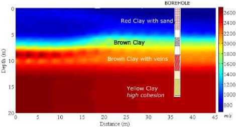
Fig. 9. Seismic tomography in Barrancabermeja refraction survey

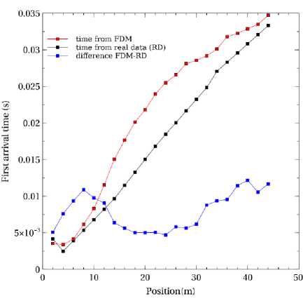
Fig. 11. Travel time for FDM and field data set in x=0m source.

The modeling allowed an analysis and study of seismic survey on models with different geometrical configurations and variation of the seismic velocity with depth. With respect to the number of geophones necessary to record the seismic events involved in seismic refractions, 24 and/or 48 geophones are sufficient, and this is a configuration similar to the standard equipment used in real seismic survey.

This type of seismic modeling allows studying the arrival times and synthetic seismograms in layered and uniform subsurface models. The application varies from verification of data inversion algorithms to the optimal seismic survey geometry determination for various structure of the substrate in complex areas.

Acknowledgement

The authors express their acknowledgment to the company of geotechnical exploration and engineering (TORRES ING S. A. S.) and Associate Professor Oleg Kovin for their recommendations to improve this work.