Simulation and calculation of heat transfer in multilayer wall structures based on iterative models

Цитирование: Жакатаев, Т. А. Моделирование и расчет теплопередачи в многослойных стеновых конструкциях на основе итерационных моделей / Т. А. Жакатаев, К. Какимова, Л. Таукенова, Т. Сериков // Журн.Сиб. федер. ун-та. Техника и технологии, 2022, 15(5). С. 622–633. DOI: 10.17516/1999-494X-0410.

and the last layer of wall t_{w , n +1} . That is, these two temperatures can be calculated during iterative calculations. Same as all internal layer temperatures. In all previously known classical cases, usually these two temperatures are set as known, predetermined.

The first, internal liquid and external liquid (or gas) are fluids. Their respective temperatures t f _,1 , t f _,2 are set as known. Thus, the iterative task starts under the not precisely defined boundary conditions of the 1st, 2nd and 3rd genera. These boundary conditions are determined approximately. The heat exchange between these liquids and the contacting solid surface may be either forced or natural convection. This is the nonlinearity of the problem we solve.

You can only specify initial approximations for α ₁ and α ₂ . Then, all values of t_{w , i} and α j , i = 1,2,3,…, n + 1; j = 1,2. In the case of convective heat of return, the mutual dependence is expressed

/ Pl’ , \ by the coefficient , where Prf, j is the Prandtl number at either the first or second liquid V'Tw.J "

temperature, Prw, l – Prandtl number at either the first or last wall temperature, k – is a fractional, non integer number. In the case of free convection, mutual dependence is expressed by means of the Grasthoff number. Which is included as a coefficient in the formula for the Nusselt number. (Grm)k, a3 . . . .

Glm — 9 Pf ~T (tf,j — twj') , k – fractional, not an integer. The nonlinearity of the problem follows from the fact that in the formula qj = αj ( tf _, j – t_{w ,} j ) heat transfer coefficient αj itself is a non-linear function of ∆ tj = ( tf _, j – t_{w ,} j ), αj = f (∆ tj ), j = 1,2, for the first liquid and for the second liquid. In the case of a wall of n layers on the side of the second external liquid t_{w ,} j = t_{w , n +1} .

As our computational practice has shown, such a problem can be solved at given only temperatures of the first internal and external external liquid. For a wall of n-solid intermediate layers, this task is given to the system of q_{n +2} heat flows for n + 1 unknown values of solid wall temperatures t_{w , i} , i = 1,2,3,…, n + 1.

When equating the values of thermal flows q i = q i +1 , i = 1,2,3,…, n + 1, the system of equations becomes closed, complete: n + 1 equations for n + 1 unknowns t_{w , i} , i = 1,2,3,…, n + 1.

A closed system of equations can be solved by substitution methods, that is, the gradual elimination of unknowns. However, this path has the inconvenience that as the number of layers of the wall n increases many times, the transformations for the equations of the system become more complicated. To determine from them all the temperature values of the walls t_{w , i} in the form of an explicit formula.

Adjusting to the final result becomes a very tedious task for manual transformation of equations. Explicit expressions in the form of formulas for t w , i would be interesting and useful in that each of them could be used as a criterion of convergence of the iterative process. Currently, there is a growth and diversity of computer computing programs and tools. These programs tend to greatly simplify the user interface.

It comes to the fact that soon at the level of game tasks, some computational algorithms and programs will be able to be compiled by secondary students in general education schools. Therefore, specific expressions for t_{w , i} in the form of formulas would be very useful precisely in terms of performing thermal calculations at the level of such simple user interfaces and simple computers.

Without using powerful software tools such as matlab, matcad and others. They require sufficient powerful computers, a processor, and RAM. Among others, we are also trying to make computational capabilities available to a wide range of engineers and technicians. And on any simple computer. Among others, an accessible and easily operated Qbasic64 program can be recommended.

Heat transfer processes play a critical role in all technical and technological processes [1–12].

There are a large number of problems that are solved by accurate analytical and sex analytical methods [1–16]. However, at present, a new direction attracts increasing attention of researchers – methods of iterative solutions of nonlinear boundary conditions in problems of heat transfer through one and multiple-layer walls [17–20].

In [17], the problem of heat transfer through an extended pipeline is solved. This is the task of heat transfer in the system: coolant-pipe – external medium under variable boundary conditions. When the internal medium (coolant) and the external medium (cooler) is service water.

Publication [18] shows a solution to the problem of cooling the liquid in a heated cylindrical vessel under variable boundary conditions, when the temperature of the heated liquid, the walls of the vessel and the heat flows change continuously over time. In these works, the wall of the pipe and the cylindrical vessel appear to be single layer. Therefore, unlike these works, we will consider solving similar problems through multi-layer walls. The thermophysical parameters of the walls (density, coefficient of thermal conductivity, heat capacity, etc.) can vary depending on the temperature, χ_i = χ_i ( t j ). In works [17–20], the heat transfer problem is solved taking into account the nonlinearity expressed through α j = f (∆ t j ). That is, the roots of nonlinear equations are calculated by iterative numerical methods. Values of t w , i serve as unknown values of calculated roots. Iteration is carried out based on refinement of their values.

Let’s start by solving the problem for a flat wall of one layer, n = 1 in Figure 1. The object is set in such a way that only the temperatures of the 1st internal liquid t f ,1 and the temperature of the external 2

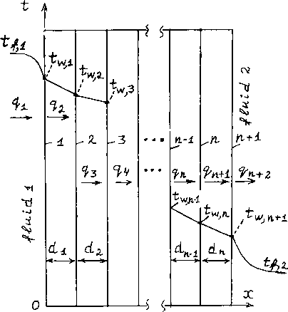
Fig. 1. Heat transfer in a system: the heat carrier (environment 1) – a flat wall from n-layers – the external environment-2

liquid t f _,2 are known. Heat transfer proceeds from the heated medium 1 through the wall to the medium 2. Thus t f _,1 >  t f _,2 . The problem is nonlinear if, at the beginning of the process, the temperatures of the first (inner) t w ,1 and second (outer) walls t w ,2 are unknown. They are then determined during iterative calculations on a computer.

Theoretical decision

Let’s consider a stationary heat transfer:

where α1, α2 – coefficients of heat transfer from the 1 liquid to the wall surface 1 and from the wall 2 surface to the external cooling medium 2, qi – density of heat flows (i = 1,2,3), W/m2, λ-coefficient of the wall thermal conductivity,      , d – wall thickness, m.

,,                                                  ,

Consider the system (1) – (2), q ₁ = q ₂ . From here we find the expression for t_{w ,1} :

_ «11/4    pt_W 2 wA p-vct^   p+a^ ^,

where = λ / d .

Consider now system (2) – (3), q ₂ = q ₃ . From here follows

Pt_w,l P^w,2 — ^a2^fw,2 ^а2^[,2 .                                       (5)

Let’s substitute (4) in (5) and after some transformations we get

^w,2

paitfl a2tf,2^P+«i)

.

The system (1)-(3) can be solved in reverse order. From the joint system (2) – (3) we find t_{w ,2} :

,    _ P^W,l+a2t/,2

lw.2                   '

’ p+a2

Consider system (1) – (2):

Let’s substitute equation (7) in (8) and get

_ ait_fil(.p+a₂)

w'^ pa2+pa1+a1a2

P«2tf,2

.

Formulas (4), (6), (7) and (9) represent a solution to the problem. They express unknown wall surface temperature values as a function of the temperature of the first and second (external) liquids and even through recoil heat factors

where k = 0, 1, 2, 3… is the iteration index.

When α_i = f (∆ t_i ) the system (10) is solved jointly in an iterative manner.

The initial values of ^w,l , ^w,n+l are given for practical reasons. Can be accepted when running from left to right

(0)     t/,l+t/,2

,

(0) _ ^1^2 – and when running from right to left.

When deciding on the computer, the limit of calculation accuracy (iteration) is taken

Let us now consider heat transfer from the internal heated heat transfer liquid to the external heat receiving liquid through a wall of two layers with different thermos physical properties. In this case, n = 2 in Figure 2.

The equations for heat flux density in this case are:

41 al " (^/,1   ^w,l) ,(12)

42        (^w,l   ^w,2^,(13)

4'1 — "Г' (tw,2 — ^И7,з),(14)

41 = a2‘ ^w,3 — t/,2),(15)

w

λ1, λ2 – coefficients of heat conductivity of the first and second wall,        , d1, d2-are thickness of the first and second wall, m.

By q ₃ = q ₄ solving the joint system (14) – (15), we express t_{w ,3} as a function t_{w ,2} and tf _,2

where P2 — ^2/^2 . Next, consider the system (13) – (14), q 2 = q 3 . We find from it tw ,2 as a function tw ,1 and tf ,2

_ Pl^w,l+(P2a2/z2)^/,2 ■

,                                                            (17)

Pl+P2-^ ²/z₂)

where z₂=a₂+ p₂ .

Now we solve the system (12) – (13), q ₁ = q ₂ . From it can be expressed t_{w ,1} first as a function t_{w ,2} , and then using (17) as a function tf _,1 and tf _,2 .

^w,l -

Oltpi + ttPlP^oJ/feZg))^

Zi-(Pi/z3)

where Z1 = «1 + Pi, 2₃ = Pl + P2 - -. ^z2

Equations (16) – (18) are the solution (12) – (15) when we solve (we banish, run) boundary conditions from right to left.

You can get solutions (run) on the contrary, on the left – to the right.

To do this, we decide (12) – (15) to solve in direct order: q ₁ = q ₂ , q ₂ = q ₃ , q ₃ = q ₄ . Then, similarly (16) – (18), the values of t_{w ,1} , t_{w ,2} , t_{w ,3} are successively expressed. The formula for t_{w ,1} is (4). Next are t_{w ,2} and t w ,3 . Only in the case of a flat wall system do the racing formulas from left to right and from right to left have symmetrical, identical views. Since in this case, for a flat wall system, the heat flux densities q_i = q_{i +1} , i = 1,2,3,…, n + 1, W/m² can be equalized. However, in the case of a system of cylindrical axial symmetrical walls (systems of coaxial pipes), it will be possible to equalize only total heat flows through various selected, fixed side surfaces F_i (m²) of these cylindrical layers, Q_i = Q_{i +1} , i = 1,2,3,…, n + 1, W. A similar pattern will be in the case of a system of spherical surfaces. Therefore, for these last two cases, the running formulas from left to right and from right to left will not be symmetrical (the same), as in the case of a flat wall system.

The formula for tw,2 takes the form tw,2

(a₁p₁t_fl/z₁)+p₂t_Wi3 z₄

P2

where Z₄ = Pl + P2 - T. Finally, the formula for t_{w 3} has the following form ^,

^w,3

(a₁p₁p2tf,i/ziz₄)+a₂t_fi2 z₂-(P2/z₄)

Thus, equations (4), (16) – (20) are the solution to the problem for a wall of two different layers, which can be solved in the form of the following iterative equations:

Hence, by induction it follows that the problem is easily generalized to a wall of arbitrary n layers with various thermo physical properties (i = 1,2,3,…, n)

Based on formulae (4), (6), (9), (16) – (21), it can be seen that as the number of wall layers increases, the complexity of the computational formula for determining the temperatures of the first, last and intermediate walls increases significantly: t_{w, i} , i = 1,2,3,…, n + 1.

The computational scheme based on the iteration of the values of thermal Q^ flows is not used in a complex way for multilayer walls when n > 3. For example, for a wall of three layers of different materials, the calculation formulas are:

_ «iPlPzt/.l ^w,3 —              i ’     21222зУ1у2Уз	P3a2tf,2 D .                , Z3Z4Y3
t    _ aiPiP2P3tf,i w'4 Z1z2z3z4y1y2y3	, P3«2tf,2 . R Z3Z4Y3    3	+ z4 V-2

where

Pi

Y2

R3

_ а^^д        PlP2P3«2tf,2 Cw 1 —        “1 I
'          zx	ZiZ2Z3Z4y1y2y3
_ atp^f ! ^w.2 —	P2P3a2tf,2
'     Z1Z2Y1Y2	Z2Z3Z4Y1Y2Y3

= Pi + аг, z2 = px + p2, z3 = p2 + p3, z4 = p3 + a2,

d;              ' ±          z4z2 ' °          z3z4

= 1^-, P1 = l+^^, P2 = l+^,

У1 Уз z2 z3               Z4 Z2 У1 y2               Z2 У! y2

= 1+^.

Z2 У1У2

Equations (23)–(26) are also nonlinear because the values of t_{w ,1} , t_{w ,2} ,···, t_{w , n +1} are arguments of the function of heat transfer coefficients α 1 and α 2 . Therefore, for the final solution of the problem, iterative calculations cannot be avoided. Obviously, as the number of wall layers increases, it is significantly difficult to derive formulas similar to (23) – (26). Which define t_{w, i} as explicit formulae.

The formulae (23) – (26) show that as a result of the analytical precise solution of the system of equations, all formulae for all temperatures of different walls can be found. A priori, only the temperatures of the internal and external liquids and the physical conditions of the state of these liquids are set. You can use them to define the function type for α ₁ and α ₂ . The approximate iterative algorithm reflected in the systems (16) – (26) is easily programmed.

Based on formulae (4), (6), (9), (16) – (26), it can be seen that as the number of layers of walls (n > 3) increases, the complexity of manual conversion of the original system of equations for heat flows increases significantly. To obtain direct explicit formulas for determining the temperatures of the first, last, and intermediate walls: t_{w, i} , i = 1,2,3,…, n + 1. When unknowns are sequentially excluded when substituting some equations into others. Since these equations have to be output analytically manually. The number of intermediate equations in the system (12) – (15) increases. Therefore, the resulting difficulty in manually converting equations is a limiting aspect of this method.

The system (21) – (26) can also be used for a transient process. Only in this case is it necessary that for each small time interval ∆ τ_i the conditions of temperature constancy on all walls t_i ≅ const are met. To a certain extent, approximate. Which entails q_i ≅ const . Also approximately. When moving to the next time period ∆ τ_{i +1} these values will change in the form of a step function. With a small fixed change step.

However, the most optimal, convenient and practical method turned out to be the method of bringing the above problem to a nonlinear expanded system of algebraic equations:

(«1 + Pi) • tw l — рг • tw 2 + 0-tw3 + ■■•+0	" tuz,7l+l - al "  tf,l ,
Pi ■ tw,i - (Pl + p2) ■ tw2 + p2 • tw3 + 0 ■ twA + •	■• + 0 ■ twn+-^ — 0,
о ■ twA + p2 ■ tw>2 - (p2 + Рз) ■ tw3 + p3 ■ twA+ 0 "  А,1 + '" "*" Pn-1 ' ^w,n-l — (Pn-1 + Pn) " tw,n	+ о ■ tW] n+i — 0, "\"Pn " ^MZ,n+l — 0,	(27)

О " ^w.l "*" '■' "*" О ■ t_w>n_i - р_п ■ t_wn + ((Z₂ + Pn) " tw,n+l *^2 " ^/,2

The system (27) can be written as a matrix equation

(а1+Р1),-Р1, 0,  -, 0 Pi, - (Pi +P2), P2-O- ••• >  0 0, Р2.ЧР2 +Рз)> Рз,0,---,0	*	tw,l A,2 ^w,3		«1 • t/,1 0 0	.                       (28)
O-"'.Pn-l.-(Pn-l+Pn). Pn)		^w,n		0
0,-, 0, 0, -pn,(«2 +Pn)		^W,?l+1		a2 ■ tf,2

Calculation results in Matlab

According to the calculation equations (27), (28), calculations were made for a flat wall of two layers: calm water – reinforced concrete wall (first layer) – metal wall, skin (second layer) – air.

Heated water temperature tf ,1 = 80.0 °С, outside air temperature tf ,2 = 10.0 °С, first wall thickness d 1 = 0.06 m, thermal conductivity λ 1 = 1.55 W/(m· ^o C), second wall thickness, iron material skin layer d 2 = 0.03 m, λ 2 = 0.055 W/(m· ^o C), α 1 = 350.0 W /( m ² ∙ °С), α 2 = 6.6 W /( m ² ∙ °С).

Under these conditions, numerical iterative calculations show the following values: t_{w 1} = 79.729 °С, tw 2 = 76.060 °С, tw 3 = 24.360 °С, q 1 = q 2 = q 2 = q 4 = 94.782 W / m ² .

Consider convective heat transfer between a solid surface and a streamlined liquid. In this case,

.              (PrA°'25

the Nusselt number includes the multiplier, the next coefficient [1–20] ^zi — I— I . The effect of \Piw'

changing the wall temperature t_w is taken into account by changing the value of the Prandtl number Prw . As a function of temperature Prw = f ( tw ).

In the case of the first calculation, iterations for α 1 we deliberately make an error and take tw 1,0 = 60.0 °С. That is, a deliberate error, the deviation from the truth is δtw 1,0 = 20.0 °С. Accordingly, the variation z 1 will be 0.92 ≤ z 1 ≤ 1.0. Accordingly, the variation of the Nusselt number Nu will be δNu ≈ 8 %. The corresponding variation (change) δt_{w 1} ≈ ±1.6 °С. It can be seen that in a small, finite number of iteration steps it is possible to achieve the required accuracy of the calculation scheme. If not exactly at first, the first values of α ₁ and t_{w, 1} were not set correctly.

Heat transfer through multi-layer cylindrical walls

Let us now consider the heat transfer through the multi-layer cylindrical walls. In cross-section, this pattern will repeat Figure 1 and Figure 2. Slightly to the left of the point O (Fig. 1), the axis of symmetry of the long pipe OZ will pass. Up, parallel to axis t. In this case, it is possible to equate not the power flows (W), but the linear densities of the thermal energy flow, ^l = ~ ,

Чц —

27гЛ(Д([

.

di

When you move from one surface to another,

Qi,i — Qu — ■" — qi,n — Qi.n+i .                                           (29)

The power flow W densities q ( W / m ² ) will not be constant. When you switch from one surface to another cylindrical surface. The complete system of equations expressing the law (29) will have the form (27) and (28). The only difference is that the p_i coefficients now have the form

_ 2лХ^

Pi — di+1 .

Follows from the theory of dimension that values α ₁ and α ₂ will be written with new coefficients CC^ — TCd^OC-^ , ^a2 ^— T^[d-n+'L^a2 , W/m. Thus, the cylindrical problem is solved in the same way as a flat one-dimensional problem. For the heat flow system.

Heat transfer through multilayer spherical walls

Figure 2 shows a multi-layer spherical wall.

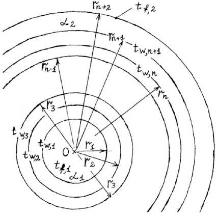
Fig. 2. Multilayer spherical wall

In this case, the task is slightly complicated. When moving from layer to layer, the following

J             W physical values cannot be equated with each other: raft of energy flow j, , power flow density, , linear power density, W/m. However, we found a solution. It is possible to equate the total power W that flows through these closed spherical surfaces

Qi — Q2 —    — Qi — ■•■ = Qn+i,                                     (30)

where _Ql = „^11^1 Mt , W.

Based on (30), you can obtain the following system of equations for a wall from many spherical layers

(«1 + Pi)t_w4 - p_Tt_w-2 + 0 ■ t_w-3 + ••• + 0 ■ t_w>n+1 = aVf.i,

Pit_wA - (Pi + p₂)t_w2 + p₂t_w3 + 0 ■ t_wA + - + 0 ■ t_w>n+1 = 0,

0 ■ t_wA + p₂t_w>2 - (p₂ + p₃^t_w3 + p₃t_wA + 0 ■ t_WiS + - + 0 ■ t_w._n+1 = 0, (31) Pn-ltw.n-l - (Pn-1 + Pn^w.n + Pntw.n+l = °,

• ^—Pn^w.n + (^2 + Pri)tw,n+1 ^— Ct2^f,2 •

Thus, problem (30) based on the system of equations (31) led to task (27), (28). We proved that in this way it is solvable. In the case of a system of spherical walls Pi - ЯЛ;^¹¹, 5_Z = ^=±1-^2, dt = 2Г;, di = 2r_z – diameter of the i-th wall of the spherical layer, m, δi – thickness of the layer, m, «1 = «1 ■ Pi, «2 = «2 ‘ F_n+1 – new coefficients in the system (31).

Conclusions

• 1.    By the method of excluding unknowns from the system (27), it is possible to sequentially obtain defining equations for all values of t w, i . Thus, analytical formulas are obtained that allow iterative calculations of wall temperature from one to three layers and, respectively, five heat flows. In this case, only the temperature values of the internal (heat transmitting) and external (heat receiving) liquids are initially set.

• 2.    With a further increase in the number of layers of walls (n > 3), the establishment of explicit formulas for t_{w, i} becomes bulky and difficult to implement with a manual transformation of the system of equations. Formulas (21) – (26).

• 3.    The practice of computing has shown that the most convenient is to bring the problem to a closed and defined system of (n + 1) – equations for (n + 1) – unknown values of the temperatures t w, _i of the walls. Expanded system of equations (27), (28). This system of equations is easily calculated in the mass-accessible packets to which Matlab belongs.

• 4.    It has been proved that in the case of a system of cylindrical and spherical walls, the problem is also solvable. A similar system of equations is obtained, as in the flat case. With new coefficients that allow you to save balance equations for heat flows.