Simulation of electric power plant performance using Excel®-VBA

Published Online May 2018 in MECS

Electricity is produced in large quantities at various electric power plants by converting different forms of energy such as fossil fuels, nuclear energy, water power, etc. Modern economies depend on electrical energy to sustain their pace of activities in virtually all sectors [1]. The Nigeria power system has being in a state of epileptics for more than two decades [2]. This experience unfortunately is fraught with a very weak electrical sector that is characterized by inadequate generation amongst others. The whole electric power sector is no longer engineering oriented; no effort is being made to ensure proper study of the whole sector and makes operation carried out properly. Being able to do these require both man power and tools. Beside, Transmission Constrained Generation Expansion Planning(TC-GEP) problem includes decision on site, capacity, type of fuel of new generation units, which should be installed over a planning horizon to meet the demand of energy expectations [3]. Complexity arises when practical generators constraints (prohibited zones, valve point effects, pollution control) are taken into consideration [4].

Simulation is a process of imitation or generating reality or things that may not be achieved, or for some reasons didn’t accomplish in the real world. Simulation is an indispensable problem-solving methodology for the solution of many real-world problems [5]. In this paper, the simulation tools will be used. The act of simulating something first requires that a model be developed; this model represents the key characteristics or behaviors of the selected physical or abstract system or process [6]. The model represents the system itself, whereas the simulation represents the operation of the system over time [7].

The act of simulating generally entails representing certain key characteristics or behaviours of a selected physical or abstract system. Key issues in simulation include acquisition of valid source information about the relevant selection of key characteristics and behaviours, the use of simplifying approximations and assumptions within the simulation, and fidelity and validity of the simulation outcomes [8]. Simulation is the imitation of the operation of a real-world process or system over time [9].

Simulation is used in many contexts, such as simulation of technology for performance optimization, safety engineering, testing, training, education, and video game [10]. Simulation is also used with scientific modeling of natural systems or human systems to gain insight into their functioning [11]. Simulation can be used to show the eventual real effects of alternative conditions and courses of action. Simulation is also used when the real system cannot be engaged, because it may not be accessible, or it may be dangerous or unacceptable to engage, or it is being designed but not yet built, or it may simply not exist [12].

A generator is a machine that transforms mechanical energy into electric power. Operation of electric power system involves excitation of the current of synchronous generator which is the main source of reactive power [13]. Prime movers such as engines and turbines convert thermal or hydraulic energy into mechanical power. Thermal energy is derived from the fission of nuclear fuel or the burning of common fuels such as oil, gas, or coal. The alternating current generating units of electric power utilities generally consist of steam turbine generators, gas combustion turbine generators, hydro (water) generators, and internal-combustion engine generators [14].

The simulation of power plant requires the generation of failure and repair events that occur in a random manner that may be represented by specified probability density functions [15]. In the case of power station the failure event occurs with the theoretical assumed distribution that is exponential. Similarly, the repair event must be generated with time to repair that is also satisfied the exponential. Algorithms for generating these random events will be developed in this chapter. In addition, Graphics User Interface (GUI) is defined and designed to enable the user to easily run the simulation without having an experience with spreadsheet directly.

In this research, a tool for simulating of electric power plant performance is addressed. This tool will help power station operators to study, better understand their facilities and be able to plan operations efficiently. Some of the useful tools are;

• i.    data acquisition systems logging condition on a continuous basis;

• ii.    analytical tools for forecasting and guiding the operations of electric power plant;

• iii.    planning software for operations and maintenance; and,

• iv.    modeling and simulation can also be considered as tool.

• II.    Aim and Objectives

The aim of this research study is to develop a tool that will enable an operator to simulate the reliability working of a power station. The objectives of the work are to:

• i.    identify the procedure for generating random events that will simulate failure and maintenance events for Turbo-alternator;

• ii.    develop the necessary programming structures to enable realization of the simulation module using the Excel – VBA, and;

• iii.    create a Graphics User Interface (GUI) to facilitate easy and friendly data entry and interaction with the simulator

• III.    Methodology

The methodology adopted to carry out this research work was divided into these phases

• i.    utilization of pseudo-random numbers to generate exponential mean distributed, Time Between Failure (TBF) and Time To Repair (TTR) events for Turbo-alternator;

• ii.    Excel VBA User-form is employed in developing the Graphics User Interface (GUI) using ActiveX Control of the toolbox for the entry of data and selection of the event to be simulated, and;

• iii.    use of interactive analysis tools to analyze and improve the performance of electric power plants.

• A.    Description of MTBF and MTTR

Mean Time-Between Failure (MTBF) and Mean Time-To Repair (MTTR) are two important aspects in Simulation of Power Plant Generator.

Mean Time-Between Failure(MTBF) is the predicted elapsed time between inherent failure of a system during operation [16]. MTBF can be calculated as the arithmetic mean (average) time between failure of a system. The definition of MTBF depends on the definition of what is considered a system failure. For complex, repairable systems, failure and repairs are considered to be those out of design conditions which place the system out of service and into a state for repair [17]. Failures which occur that can be left or maintained in an unrepaired condition, and do not place the system out of service, are not considered failures under this definition [18].

Failure Rate : The mean (arithmetic average) number of failures of a component or system per unit exposure time. The most common unit in reliability analysis is hours (h) or years (y). Therefore, the failure rate is expressed in failures per hour (f/h).

This creates a fundamental issue, since the use of constant MTBF and Failure Rate in reliability analysis is based upon the assumption that the probability density and distribution functions for the time between failures are exponential.

Mean Time-To Repair (MTTR) is the average time that it takes to repair something after a failure. For something that cannot be repaired, the correct term is “Mean Time-To Failure” (MTTF).

Some would define MTBF – for repair-able devices – as the sum of MTTF plus MTTR. (MTBF = MTTF + MTTR). This distinction is important if the repair time (MTTR) is a significant fraction of MTTF.

• B.    Development of Randomly Occurring Fault Events

The failures of a turbo-alternator are in general described by Weibull distributions which more accurately reflect the early mortality, mid-life and ageing characteristics of natural systems. In this work, only the mid-life performance is assumed and this as earlier stated satisfy exponentially distributed density functions. The algorithm thus must generate random mean-time-between-failures that are exponential.

The random number generator for the EXCEL worksheet with its VBA add-in are used to generate a sequence of cumulative density function values that are then inverted to give the corresponding MTBF by using the formula:

TBF = —ln(1 — rand) /

where ’rand’ is generated by the worksheet with values ranging between 0 and 1 and λ is the lamda-failure rate. Again this same random number generator for the EXCEL worksheet with its VBA add-in are also used to generate a sequence of cumulative density function values that are then inverted to give the corresponding MTTR by using the formula:

TTR = —ln(1 — rand)/

where ’rand’ is also generated by the worksheet with values ranging between 0 and 1 and µ is the miu-repair rate that satisfied the desired output. The algorithm provides the logic for controlling the number of trials whilst the selection and definition of parameters are managed by User-forms. The design of the User-form is treated in section 3.3. The algorithm may be represented by the following flow diagram.

• IV.    Design, Testing and Analysis

Given the structure of the problem, the design specifications incorporate the control elements that permit the name of power station/identification, investigator’s name, investigation date, Specification of the number of turbo-alternators, Specification of the parameters of turbo-alternators, Specification of the number of cycles/iteration to be performed and Specification of the file to store results. The design mode includes generator number, failure and repair rate, repair rate, year installed, and rated output as shown in Fig 1 and 2.

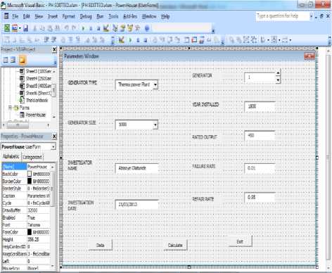
Fig.1. GUI Design mode

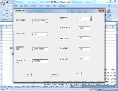
Fig.2. GUI Running mode

Tests of the different stages were carried out and the verification of performance is implemented and the results are shown in Fig.3.

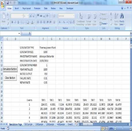
Fig.3. GUI Simulation Result on the Microsoft Excel Worksheet

The success of a simulation depends on the quality of its random event generators and the number of simulations that have to be run before a representative process can be said to have been arrived at. It was decided to study the distributions of the random failure events which the algorithm. The simulations were used to generate as many as 500 failure events. These events were then catalogued and organized into a number of intervals derived using 100 samples as the basis.

• V.    Results and Discussion

Iterations for 25, 100 and 250 samples were performed and the cumulative distributions were determined.

• A.    TBF Cumulative Distribution

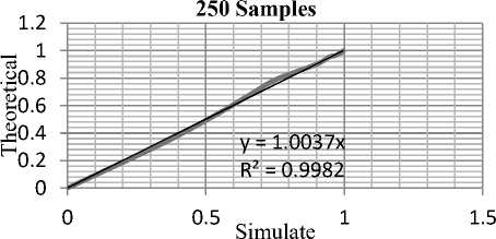
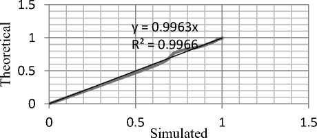
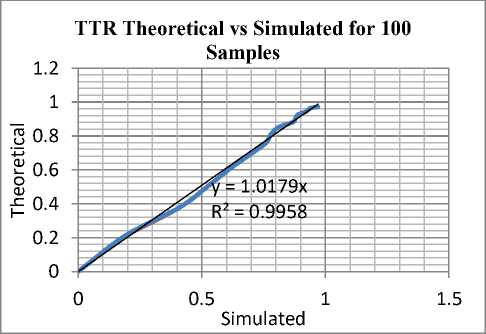
The cumulative relative frequency functions for each sample set was determined. A corresponding set of values were determined for an exponential distribution with the same mean value. These were then plotted to study the corresponding correlations between the observed and the calculated values in Fig.4, Fig.5 and Fig.6. The graphs for the cumulative relative frequencies/distribution functions are presented while the correlation diagrams are show in Fig. 7, Fig. 8 and Fig. 9. It can be seen that at the low sample end the curves exhibit very unsteady features which translate into very poor correlation between the theoretical and the observed values. However beyond 250 samples the set of random events observed seem to represent a good fit. The coefficient of correlation beyond 100 samples was greater than 99.6%. Any study attempting to duplicate the workings of an exponentially distributed random process using this EXCEL-VBA engine would give very satisfactory results for over 100 runs. The shapes of trend curves can be seen to converge slowly to an exponential form although confirmation of this must be ascertained by statistical or other methods. The shapes appear to become more regular as the number of samples increase.

TBF Theoretical vs Simulated Plot for

TBF Cumulative Relative Distribution

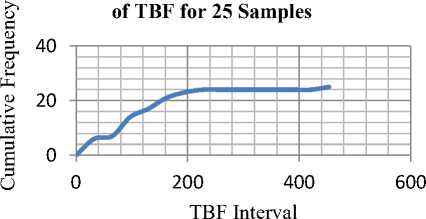
Fig.7. Cumulative Relative Distribution of TBF for 25 Samples

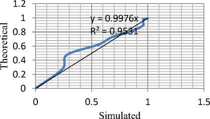
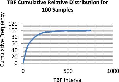
Fig.8. Cumulative Relative Distribution of TBF for 100 Samples

TBF Theoretical vs Simulated for 100 Samples

TBF Cumulative Relative Distribution

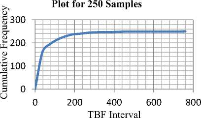
Fig.9. Cumulative Relative Distribution of TBF for 250 Samples

• B.    TTR Cumulative Distribution

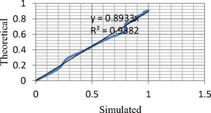
In order to confirm the conclusion even for the repair events, a similar exercise was carried out using the repair rate. The results are as shown in Fig 10 through Fig. 15.A similar analysis shows that the correlation is better than 99.5%. This implies that 100 repetitions of the process should give a very satisfactory simulation. Indeed even the case of 250 samples yields a corresponding correlation of 98.8%. Since it is enough to work with 95% confidence, it may be possible to generate a simulation with as few as 25 trials

The cumulative distribution is simply the cumulative number of failure and repairs one might expect over a period of time. The relative rates at which TBF and TTR are added to the cumulative distribution remain constant. However, as the population declines as a result of failure and repair events, the actual number of mathematically estimated events decreases as a function of the declining TBF and TTR. As the frequency of simulated TBF and TTR distribution asymptotically approached zero, the cumulative relative frequency curves asymptotically approached total number of each sample, that is, 25, 100, and 250.

TTR Theoretical vs Simulated for 25 Samples

TTR Theoretical vs Simulated Plot for 250 Samples

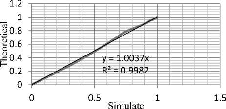
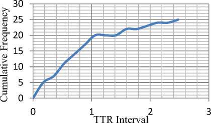
Fig.13.Cumulative Relative Distribution of TTR for 25 Samples

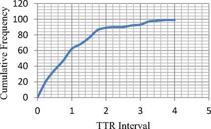
Fig.14.Cumulative Relative Distribution of TTR for 100 Samples

Studying the charts for the theoretical against the simulated for both the failure and repair events in Fig.4, 5,6 and 10,11,12, the graph lines for 25 samples have more contours than that of 100 samples. Likewise, the graph line for 100 samples has more contours than that of 250 and so on. It was discovered that as the number of samples are increase as a result increase in number of random number generated, the lines of charts were nearly becoming straight lines. This shows that the correlation between theoretical exponential and the Monte Carlo simulated charts of 25 samples is more poor comparing to that of 100 samples and that of 250 samples is more better. It also tells us the point at which the results of the simulation will approach exponential distribution.

Average Output Performance of Turbo-alternator Operation over 12-

M onth Time Horizon for 25 Samples

1.2

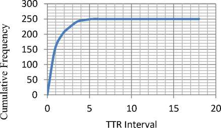
Fig.15.Cumulative Relative Distribution of TTR for 250 Samples

0.8

0.6

0.4

0.2

0 Plant

Condition

Time Axis

Up = Plant Condition 1 Down = Plant Condition 0

Fig.17. Simulation Plot of Average Output of Turbo-alternator operation for 25 Samples

• C.    Failure and Repair Time Horizons

0.8 0.6 0.4 0.2

The charts in this section show a time horizon of up and down time of a Turbo-alternator over 365 days (12-Month). The X axis represent the result of TBF and TTR up to 365 days, while the Y axis represents up (working/TBF) period is when the line is on 1 and the down (waiting/TTR) period is when the line is on 0.

Fig.16 shows the output of performance of a TurboAlternator when the average of TBF and TTR have not been taken. While Fig.17 shows the output performance of the same Turbo-Alternator after taken the average. The likely up and down time in Fig.17 is of higher degree of tendency in comparison with Fig.16.

The analyses of simulation show that the failure and the repair events of any Turbo-Alternator agreed with the pre-assumed exponential density function. They show that those failure and repair events occur at the mid-life as also pre-assumed. In addition, the up and down time of the Turbo-Alternator will help the policy makers and the operator to make decision as regard to the power plant.

1.2

Up = Plant Cond ition 1 Down = Plant Condition 0

_Plant 0      100     200     300     400

Condition              Time axis

Fig.16. Simulation Plot of the Turbo-alternator operation

• VI. Conclusion

This report presents the results of an effort to simulate a power station whose turbo-alternators have exponential failure characteristics and repair rates. The procedure is implemented in EXCEL-VBA, a powerful augmented spreadsheet with a macro language enhancement. Random events generated using the functions in the software were created and tested for compliance with the desired exponential distribution. It was found that as the number of samples increased the behavior of the random events better represented the desired form with a correlation of almost 99% for 25 trials. This corresponds to a confidence interval of better than 95% and hence should be used as the median for practical applications.

The result of this Simulation shows that the failure of each generator exhibits exponential distribution. This is characterized by constant failure rate, stochastic process and independent failure times. This situation happens when a generator is in the useful life period and operated beyond the infant mortality stage and is yet to get into the wear out stage. Therefore, Simulation can allow analysis of a multitude of different reliability and maintainability aspects of Turbo-alternator such as the identification of weak points and the assessment of power plant upgrading better performance.

The resulting software package has also a graphics user interface (GUI) which serves as a very helpful means of insulating a user from the complex workings of the software.