Simulation of wind speed in the problems of wind power

The revival of interest in the use of wind power is now connected with the opportunity to determine the feasibility of converting it into electricity. Economically, this occurs when the feasibility of wind speeds exceeding 5 m/s. And this imposes a significant limitation on the development of wind energy. An area which has a rich wind, as a rule, do not need in electricity because of remote location of industrial facilities and residential areas.

Most wind turbines are used to generate electricity in power grid, as well as offline. When the wind speed u ₀, air density ρ and swept area A, wind turbine has an output power [1]:

3 ρu P = C A —0, p 2

where С_р is the fraction of the upstream wind power, which is captured by the rotor blades andcalled the power coefficient of the rotor or rotor efficiency.

From (1) can be seen that the power P is proportional to the swept area A and the cube of the velocity u 0 . Power coefficient С р depends on the design of rotor and wind speed. Since the wind

From the expression (1) we can see that the wind speed is the most critical data needed to appraise the power potential of a candidate site. The wind is never steady in any state. It is influenced by weather conditions, topography, and relative height above the surface. The wind speed varies by the minute, hour, day, season or year. Therefore, the annual mean speed needs to be averaged over 10 or more years. Such a long term average raises the confidence in assessing the energy-capture potential of a site. However, long-term measurements are expensive, and most projects cannot wait that long. In this situation, the short term, say one year, data is compared with a nearby site having a long term data to predict the long term annual wind speed at the site under consideration.

Mathematical model of wind speed

Probabilistic model of the wind speed

The variation in wind speed are best described by the Weibull probability distribution function ‘h’ with two parameters, the shape parameter ‘k’ and the scale parameter ‘c’. The probability of wind speed being ‘u’ during time interval is given by the following expression [2]:

h ( u ) = ( ^k )( ^u )^{( k - 1)} e cc

-

(u)k c , 0 < u < ∞.

Fig. 1 is the plot of h versus u for three different values of k. The curve on the left with k=1 has a heavy bias to the left, where most days are windless (u=0). The curve on the right with k=3 looks more like a normal bell shape distribution, where some days have high wind and equal number of days have low wind. The curve in the middle with k=2 is a typical wind distribution found at most sites. In this distribution, more days have lower than the mean speed, while few days have high wind. The value of k determines the shape of the curve, hence is called the “shape parameter”.

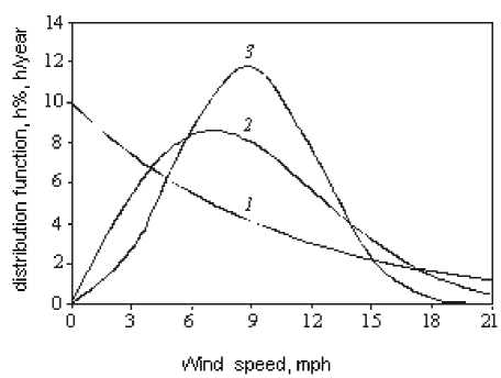
Fig. 1.Weibull probability distribution function with scale parameter c=10 and shape parameter k=1,2 and 3 (plots 1-3 respectively)

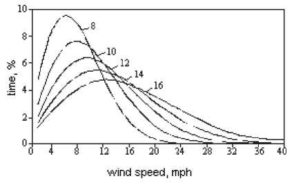
Fig. 2. Weibull probability distribution with shape parameter k=2 and the scale parameters ranging from 8 to 16 miles per hour (mph)

wind speed, mph

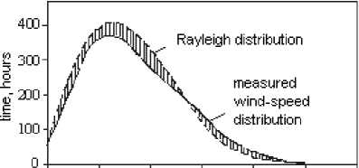
Fig. 3. Rayleigh distribution of hours/year compared with measured wind-speed distribution

The Weibull distribution with k=1 is called the exponential distribution which is generally used in the reliability studies. For k=3, it approaches the normal distribution, often called the Gaussian or the bell-shape distribution.

Fig. 2 shows the distribution curves corresponding to k=2 with different values of c ranging from 8 to 16 mph (1 mph = 0,446 m/s). For greater values of c the curves shift right to the higher wind speeds. That is, the higher the c, the more number of days have high winds. Since this shifts the distribution of hours at a higher speed scale, the c is called the scale parameter. At most sites the wind speed has the Weibull distribution with k=2, which is specifically known as the Rayleigh distribution.

The actual measurements data taken at most sites compare well with the Rayleigh distribution, as seen in figure 3. The Rayleigh distribution is then a simple and accurate enough representation of the wind speed with just one parameter, the scale parameter ‘c’.

Summarizing the characteristics of the Weibull probability distribution function:

k = 1 – makes it the exponential distribution, h = λe^–λu , где λ = c ^–1;

k = 2 – makes it the Rayleigh distribution h = 2 λ ² ue^{– ( λu )2};                       (2)

k = 3 – makes it approach a normal bell-shape distribution..

Since most wind speed sites would have the scale parameter ranging from 10 to 20 miles per hour (about 5 to 10 m/s), and the shape parameter ranging from 1.5 to 2.5 (rarely 3), our discussion in the – 152 –

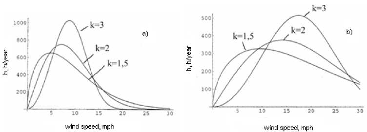
Fig. 4. Weibull distributions: а) 10 mph, б) 20 mph.

following will center around those ranges of c and k. Fig. 4 displays the number of hours on the vertical axis versus the wind speed on the horizontal axis with distributions of different scale parameters c=10, and 20 mph and shape parameters k=1.5, 2 and 3.

The resulting distribution law for any area can be used to determine the potential of wind power and annual power generation in the execution phase of technical – economic calculations.

Deterministic model of the wind speed

Mode speed is defined as the speed corresponding to the hump in the distribution function. This is the speed the wind blows most of the time.

Mean speed over the period is defined as the total area under the h-u curve integrated from u=0 to ∞, divided by the total number of hours in the period ( 8760 if the period is one year): ^ю

U = hudu .

mean 8760 1

In general, for the Weibull function can be obtained:

Umean = СГ (1 + 1) = C [(1)!](3)

k k ^,

U. == cn Г (1 + 3)(4)

mean k.

If n = 3 expression (4) can be rewrite:

U'me .an = c ’ Г (1 + 3)(5)

k from which we can to derive an expression for wind energy.

The parameters c and k are defined on the phase approximation of the Weibull distribution of meteorological observations. For example, if U_mean and U_m ³ _ean are known, the parameters c and k are defined by the equations (3) and (5). U mean and U_m ³ _ean can simply define by modern methods of primary processing of meteorological information without referring to the results of numerous individual measurements. The Weibull distribution parameter k is dimensionless.

Dimensionless parameters, allowing to operate with distribution functions, regardless of the actual values of wind speed, convenient in many cases, for example, when the average wind speed is known only. At the approximated Weibull distribution parameter k, as a rule, is in the range 1.6 ...3.0. The value c ~ 2U mean! Vn is not more than 1% different from the corresponding value in the Rayleigh distribution, when k = 2 = const, and therefore it is possible to show that:

U

mean

(W )(3 | 3 ) ^k

.

A number of studies verified the hypothesis that the value of k depends only on topography of this region and the general characteristics of the wind. Then if you know only the mean wind speed and the results of long-term meteorological observations, you can evaluate the frequency and duration of periods of calm.

For the Rayleigh distribution with k=2, the Gamma function can be further approximated to the following:

^Umean = ⁰,⁹ c -

This is a very simple relation between the scale parameter c and U mean , which can be used with reasonable accurancy. For example, most sites are reported in terms of their mean wind speeds. The c parameter in the corresponding Rayleigh distribution is then c = U mean /0,9, and k = 2. Thus. We have the Rayleigh distribution of the site using the generally reported mean speed as follows:

u 2

^{- 11} h ( u ) = -^e ^c

2 u

- (

u

e

( U      )²

mean

U mean

)2

.

Thus, the deterministic model to calculate the approximate value of power generated by wind turbines, at a certain average wind speed.

Spectral model of the wind speed

From a system point of view, the wind speed represents the main exogenous signal applied to the wind turbine and determines its behavior. Its erratic variation, highly dependent on the given site and on the atmospheric conditions, makes the wind speed quite difficult to model. Usually the thermic equilibrium of the atmosphere nearby Earth is assumed [3]. Therefore, turbulence results mainly from the friction between air and ground, due to the ground roughness. When designing wind turbine, the history of the wind speed extreme values (gusts) is considered for the mechanical structure design and also for control purposes.

Wind near the Earth’s surface is generally modeled by a spatial (3D) speed distribution. Assuming that the turbine is equipped with a vane (or yawing equipment) and that changes in wind direction are sufficiently slow, then the turbine rotor is maintained normal to the wind and wind turbine analysis requires only the longitudinal wind speed being synthesized/modeled. Thus, in the present book only scalar (1D) wind speed models will be used. As the interest here is focused on wind turbine behavior – 154 –

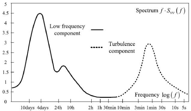
Fig. 5. Van der Hoven’s spectral model of the wind speed

in normal operating regimes, the developed models will not include extreme operating conditions like wind gusts.

Wind dynamics result from combining meteorological conditions with particular features of a given site. Thus, wind speed is modeled in the literature as a non-stationary random process, yielded by superposing two components [3 – 5]:

u ( t ) = u s ( t ) + U, ( t ), (6)

where u_s ( t ) – is the low-frequency component (describing long term, low-frequency variations); u_t ( t ) – is the turbulence component (corresponding to fast, high-frequency variations).

These components can be identified in Van der Hoven’s large band (six decades) model (Fig. 5). The spectral gap of around 0.5 MHz suggests that the turbulence component can be modeled as a zero average random process (there is little energy in the spectral range between 2 h and 10 min). u_s ( t ) is considered constant (equal to the average wind speed) when viewed at the turbulence time scale. Averaging is usually performed on a 10-min time window [3].

The low-frequency component corresponds to the very slow wind speed variations and characterizes the site from the energy viewpoint. It can be modeled as a Weibull’s distribution or a Rayleigh’s distribution see expression (2).

Fast wind speed variations (typically occurring within 10 min) are modeled by the turbulence component. This is mathematically described as a zero average normal distribution, whose standard deviation, σ, depends on the current value of the hourly average, u_s . The turbulence intensity is a measure of the global level of turbulence, depends on the ground surface roughness and is defined as:

I

t

CT u s

The mathematical description of the turbulence’s dynamical properties, ut(t), can be obtained by using two kinds of spectra: von Karman’s and Kaimal’s respectively. According to [3], Kaimal’s – 155 – spectrum reflects better the correspondence to experimental data, when turbulence is present. But von Karman’s spectrum is more consistently theoretically founded (an analytical connection with the correlation function is provided) and allows a realistic representation of turbulence data in wind tunnels. The von Karman’s model for the longitudinal component of the turbulence is:

• 4    f ■ ~

f ■ S uu ( f ) ₌ U s a 2                    I 5

,

(1 + 70.8( f ■    )²)⁶

us where Suu(f) is the power spectral density, Lt is the length of turbulence, specific to the site (ground roughness), and f is the frequency in Hz.

Kaimal’s spectral model has the form:

^f ■ S uu₂ ^{( f} ) C

4 f ■ Lb

us

(1 + ⁶ f . L ⁾⁵

us

One can note that in both models the power spectral density is influenced by the turbulence intensity, It , which determines the turbulence “level” ( i.e. , its variance, σ²) and the turbulence length, Lt , which impresses the turbulence dynamic properties (the spectral function bandwidth). Both these parameters are adopted according to various standards. For example, in the Danish standard (DS 742 2007), the following relations are used to compute these parameters:

It       Zx ln( ) z0

and respectively

150 m, z >  30 m

• 5    • zm,z <  30 m

where z is the height from ground where the wind speed is computed and z ₀ is the roughness length.

Fig. 6 comparatively presents the spectral functions at Equations 8 and 9 for the same values of parameters z , z ₀ and u_s . For an easier analysis of von Karman’s and Kaimal’s spectra, in Fig. 7a one can see the corresponding power spectral densities, S uu ( f ), whereas Fig. 7b shows the Bode diagrams of the non-integer-order shaping filter outputting the turbulence component when fed with a white noise [6].

Fuzzy model of the wind speed

Handling fuzzy information in the problems of wind energy is achieved by using linguistic variables. As part of the linguistic approach the values of variables are allowed not only the number but also the words and sentences of natural language, as well as a mathematical tool used to formalize the theory of fuzzy sets.

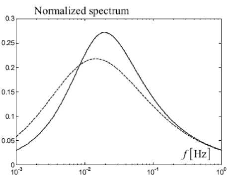
Fig. 6. Comparison between the von Karman’s (Equation 8 – solid line ) and Kaimal’s (Equation 9 – dashed line ) normalized spectra ( z =30 m, z 0=0.01 m, u s =10 m/s , Danish standard DS472)

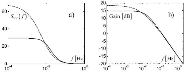
Fig. 7. Von Karman’s (solid line) vs. Kaimal’s (dashed line) spectral models (z=30 m, z0=0.01 m, u s =10 m/s , Danish standard DS472): a) power spectral densities; b) shaping filter gains

One of the main steps is to build membership functions that describe the semantics of the basic values of the variables used in the model when you create a fuzzy model of decisionmaking. These functions are characterize the uncertainty such as “approximately equal”, “average”, “is in the range”, “like an object”, etc and used to specify sets of properties.

The process of fuzzy modeling is based on a quantitative representation of the system variables in the form of fuzzy membership functions.

It is known that wind speed in the interval setting can be represented by the Beaufort scale (Table 1) [7]. At the same characteristics of the wind speed is given as both a linguistic evaluations: weak, strong, variable, etc. [8].

When information about wind speed given like an interval, for example, the wind is strong, its speed is u = [11, 14] m / s and the resulting solution of the expected power generation interval estimates are obtained, which entails a significant drawback – it is impossible to determine which value of the variable is more or less reliably.

Table 1. Strength of the wind on the Beaufort scale and its impact on wind turbines

-2 rP 'о §	45 Ph	Characteristics of wind power	Observed effects	The impact of wind on wind turbines	The conditions for wind turbines production, with an average wind speed
2	1,8 – 3,6	Light breeze	Wind felt on face, leaves rustle, vanes begin to move	not	Bad for all wind turbine
3	3,6 – 5,8	Gentle breeze	Leaves, small twigs in constant motion; light flags extended	Begin to turn lowspeed turbine	Satisfactory to the pumps and some aerogenerators
4	5,8 – 8,5	Moderate breeze	Dust, leaves and loose paper raised up; small branches move	Begin to rotate the wheel aerogenerators	Good for aerogenerators
5	8,5 – 11	Fresh breeze	Small trees begin to sway	Capacity of wind turbines up to 30% of the project	Very good
6	11 – 14	Strong breeze	Large branches of trees in motion; whistling heard in wires	Maximal power	Valid
7	14 – 17	Moderate gale	Whole trees in motion; Resistance felt in walking against the wind	Maximal power	Valid
8	17 – 21	Fresh gale	Twigs and small branches broken off trees	Some wind turbine off	The maximum permissible
9	21 – 25	Strong gale	Slight structural damage occurs; slate blown from roofs	All wind turbine off	Invalid

We use the possibility of representation of wind speed by fuzzy variables. The Beaufort scale imagines corresponding characteristic membership functions of linguistic variables of wind speed. Moreover, membership functions are chosen from the following considerations: for the border interval of values of wind speed, the famous Beaufort scale, each linguistic variable is assigned a value of belonging µ = 0.5, at these points the values of wind speed will have equal weight in relation to the neighboring variable. With a value of µ = 1 the velocity in each band is equal to ( u_max – u_min )/2 [9].

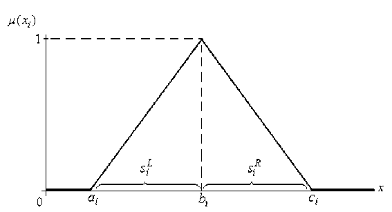
Thus, for each linguistic variable, we define the value of belonging to the whole interval (Table 2). Fuzzy numbers and intervals, which are most often used to represent fuzzy sets can be described in the form of analytical approximation using the so-called (L – R) -functions [10].

Graphically, these characteristics may be represented by a family of fuzzy triangular function (Fig. 8). From here you can see that in the section µ = 0.5, this characteristics described by the interval values, as indicated on the Beaufort scale.

Consideringthemembership functionofwind speed (Fig. 8),itisnecessarytoconsider membership in the interval from 0 to 1. So, finish the construction of each value of fuzzy variable, which will have a base value of µ = 0.

Table 2. Fuzzy variables as a characteristic of wind power

Wind speed u , m/s	Affiliations	Characteristics of wind power
1,8	0,5	Light breeze
2,7	1
3,6	0,5
3,6	0,5	Gentle breeze
4,7	1
5,8	0,5
5,8	0,5	Moderate breeze
7,15	1
8,5	0,5
8,5	0,5	Fresh breeze
9,75	1
11	0,5
11	0,5	Strong breeze
12,5	1
14	0,5
14	0,5	Moderate gale
15,5	1
17	0,5
17	0,5	Fresh gale
19	1
21	0,5

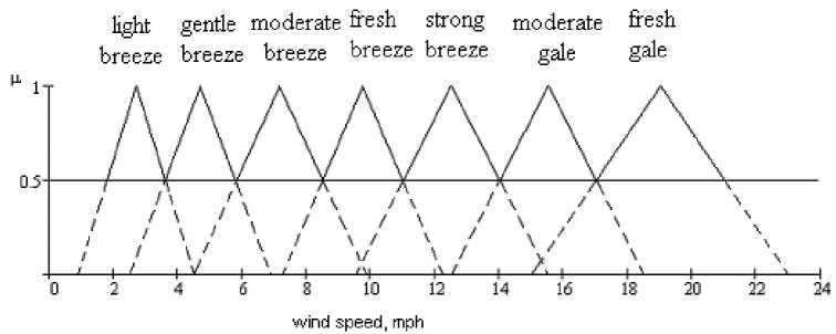
Fig. 8. Fuzzy values of wind

In general, each of these functions can be described analytically by the following expression.

м( x) = г 0, c ^ x ^ a i x-ai а

The parameters ai and ci characterize the base of the triangle, and the parameter bi – its top (Fig. 9). As you can see, this membership function generates unimodal normal convex fuzzy set with the carrier – the interval (ai, ci), boundaries (ai, ci)\{bi}, {bi} and mode bi.

si^L and si^R – left-handed and right spread of the maximum value of belonging.

In describing the fuzzy scale Beaufort, the membership function takes the form of symmetrical triangles, i.e. s _i^L = s_i^R .

Table 3 shows the values of numerical parameters (L – R) – functions that characterize the linguistic variables of wind speed.

Corresponding analytical expressions can be fined for linguistic variables of wind speed knowing the general expression (L – R) – function (12) and numerical parameters.

Often, in real problems it is necessary to split the membership function of fuzzy set on the so-called α – levels, so that if a fuzzy set A is defined on the underlying set X and α ∈ [ 0, 1 ], then the classical set Aα, defined by the expression (13), called the set of α – the level of A.

А^а  {^^ЦА⁽*)"^{а}                                                    (13)}

Figure 10 shows an illustration α – levels, α₁, α₂, … , α_n fuzzy set with a symmetric triangular membership function.

It is should be noted that, each fuzzy set can be represented by a set of α-levels. This representation of fuzzy sets used in solving practical problems, particularly in the construction of fuzzy models with different levels of fuzziness [11].

Fig. 9. Graph a triangular membership function

Table 3. Numerical parameters of (L – R) – functions fuzzy Beaufort scale

Characteristics of wind power	ai	bi	ci
Light breeze	0,9	2,7	4,5
Gentle breeze	2,5	4,7	6,9
Moderate breeze	4,45	7,15	9,85
Fresh breeze	7,25	9,75	12,25
Strong breeze	9,5	12,5	15,5
Moderate gale	12,5	15,5	18,5
Fresh gale	15	19	23

^■)

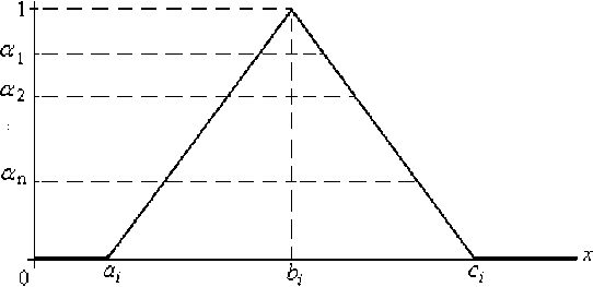
Fig. 10. α – levels fuzzy set

In further studies, the entire area of belonging from 0 to 1 should be split into multiple levels, so for clarity, will cross a few (four) points of the values of µ = (0…1);; each section (Fig. 10) will characterize the level of membership α_j.

Knowing a given level of membership and the corresponding wind speed, we can calculate the typical power produced by wind turbines with respect to a given speed, which will take place at the same α – level.

It is should be noted that when the wind speed is less than the minimum operating wind (<4m / s), blades stationary and power generated by wind turbines is zero. Thus, the values of power output of wind turbines can be determined depending on wind speed and the speed of the membership of each of the respective linguistic variable.

In general, the domain of the membership µ = (0 ... 1), we have a set of fuzzy sets Xl, where l – the number of linguistic variables of wind speed (very light, light, ... very strong).

XI ={< v2,^(v2)> , ... , < vn,^Xl(vn) >}, where n – number of levels of membership αj.

In accordance with (14) can be noted that the power of wind turbines is a function of wind speed:

Yk = f(Xl) = f {<v1,HYl⁽v1 )>< v.,HYl⁽v2)> , ... , < vn,HYl⁽vn) >}. (15) where k – a number of linguistic variable of the wind turbine power (very small, small and etc.).

Controller for improvement efficiency of wind turbine on the basis of the wind speed fuzzy model

Fuzzy modeling is a new modern technology that is used in various fields of science and technology. First of all, this technology is relevant in cases when you want to improve the adequacy of the model systems to take into account many different factors that influence the decision-making processes. In addition, mathematical models and formal management systems and processes increasingly complex and sometime system of fuzzy relations can to implement them without too much trouble [12].

In the wind power system fuzzy logic is used quite actively – fuzzy controllers used for wind turbine yaw control [13] changing the angle of attack and angle of the blade jammed, the rotor speed [14]. In this paper we propose a controller for wind turbines, which changes the blade length [15. Fuzzy model is used for realization of the wind speed, because it is most relevant in terms of impermanence energy source.

The proposed fuzzy controller is based on the idea of variable length blades, which arose as a result of the desire to increase power output of wind turbines in area 2 (area from start to rated speed of the wind turbine) [16]. The calculations showed that using of these blades can increase the production capacity up to 30%. The implementation of a fuzzy controller gives below in more detail.

The results of the development

Fuzzy controller designed for wind turbine Nordex N80/2500 kW with a radius of wheel 40 m. The study assumed that blades can be increased up to 48 m.

The length of the blade, the wind speed given by Beaufort scale and power of wind turbines are input variables for fuzzy controller. Mamdani algorithm is used for fuzzy output. The average of the maximum is used for defuzzification, which is defined as the arithmetic mean of left and right modal values. We get a specific value on which the length of blades changes to maximize power generation.

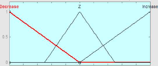
Rules were established for the proposed model – the control action (Table 4). For the linguistic variable power, P, used the following term-sets: BN – more than nominal value, SN – less than the nominal value, N-nominal value; membership functions shown in Fig. 11. For the linguistic variable wind speed, Vw, used the term-sets of the Beaufort scale; the membership functions shown in Fig. 11. For the linguistic correction of variable length, ΔL, use the following term-sets: Z – do not change, D – to decrease, I – to increase; the membership functions shown in Fig. 12.

Fuzzy controller is implemented in the program Matlab, using a special expansion pack Fuzzy Logic Toolbox. As part of this package, you can perform all actions necessary for the development and use of fuzzy models. With the help of fuzzy inference system editor FIS can set and edit the properties of high-level fuzzy inference system, such as the number of input and output variables, the type of fuzzy inference, defuzzification method, etc. We obtained a kind of summary table that can be used to assess the adequacy of the controller (see Fig. 13).

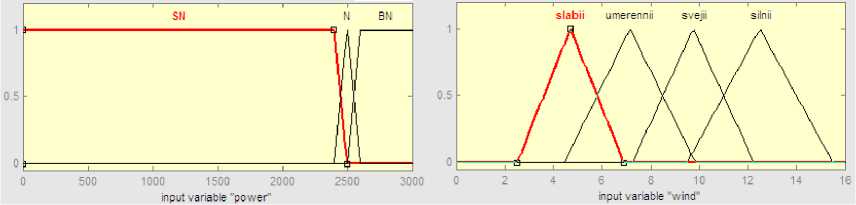
Fig. 11. Membership function for the power and the wind speed

-1 -QJ8 -0.6    -0.4    -0.2      (>      0.2     0.4     0.6     OU:;      1

output variable ”dL"

Fig. 12. Membership function to change the length of the blade

Table 4. Rules for the fuzzy controller

№ rule	Power, Р	Wind speed, Vв	Correction of the blade length, ΔL
1	BN	Gentle breeze 3,6 – 5,8 м/с	D
2	N		Z
3	SN		I
4	BN	Moderate breeze 5,8 – 8,5 м/с	D
5	N
6	SN		I
7	BN	Fresh breeze 8,5 – 11 м/с	D
8	N		Z
9	SN		I
10	BN	Strong breeze 11 – 15 м/с	D
11	N		Z
12	SN		I

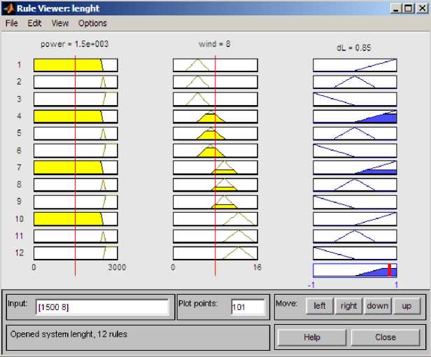
Fig. 13. Rules table in Matlab

Features of this software can also evaluate the effects of input variables on the value of the output variable.

Conclusion

In the paper reviewed the basic mathematical models of wind speed. Their area of use is defined.

Controller for improvement efficiency of wind turbine on the basis of the fuzzy logic and using wind speed fuzzy model are designed. This model tested on adequacy in Simulink/Matlab. The idea of this controller can find a place in industrial area along with existing ones. Coordination of multiple controllers, if necessary, you can also implement a fuzzy controller.