Simultaneous Image Fusion and Denoising based on Multi-Scale Transform and Sparse Representation

Published Online June 2017 in MECS DOI: 10.5815/ijigsp.2017.06.05

Image fusion is a process to take part for multi-view information into a new one image which contains high quality information. Researchers have developed algorithms based on image fusion containing high quality fused image with the help of two source images. This idea develops research area in remote sensing, medical image processing, and computer vision. Image fusion has three levels such as pixel, feature and decision level. In this paper we consider pixel level fusion [1], the fused image should keep the information and also remove the noise from the source images. The pixel level fusion is divided into spatial and transform domain [2]. The transform domain technique is used in image fusion based on multiscale transforms. It performs on a number of different scales and orientations independently.

Recently, many multi-scale geometric analysis (MGA) tools have been proposed, such as Pyramid Transforms, the Discrete Wavelet Transform (DWT) [1] - [3], the Undecimated Wavelet Transform (UWT) [1], [3], the Dual-Tree Complex Wavelet Transform (DTCWT) [4], curvelet [5], bandelet [6], contourlet [7], shearlet [8], etc. for the representation of multidimensional data. Shearlet is a new multi-resolution approach provided higher directional sensitivity properties. The authors [8] have developed shearlet with a rich mathematical structure similar to wavelets but the decomposition procedures same as contourlet transform. The decomposition process of shearlet is followed with directional filter with shear matrix whereas contourlet transform is based on the Laplacian pyramid.

The problem of dictionary learning can be stated as follows [10]:

y = Dx,DE ®тхг, x e ^rxn (1)

Where D is referred to as the dictionary matrix and x is the coefficient of matrix and both are unknown. n is the signal dimension and m is the dictionary size. The equation (1) can be solved in case of the solution to (1) is not unique when the number of dictionary element r > m (i.e. the dictionary is overcomplete). Consider the coefficient matrix x is sparse and can be observed У/ e ^mxr is a sparse combination of the dictionary elements (i.e. columns of the dictionary matrix). This problem is known as sparse coding. The learning comunity have been many works on dictionary learning. Hillar and Sommer [11] the number of sample data in fit into dictionary is exponential in r for general case. Spielman et al. (2012) sparse coding fits the 11 norm based method for undercomplete dictionary r < m . In our paper we have considered 11 norm based method r >m . The sparse coding is mainly calculated the sparsest of x which contains the fewest nonzero elements. This coding method has shown stability and efficient of algorithm Yaghoobi et al. [10] .Yang and Li et al. [11] had used sliding window technique into Sparse coding and focused on fusion process more robust than noise and registration.

A hybrid model of image fusion using MST and SR based method is proposed here where the framework is compared with different MGA method and the result is analyzed. The main purpose of this paper is to use that hybrid model for shearlet transform and sparse representation and to use de-noising method to remove any noise subjected to source images.

This paper is organized firstly for giving the theoretical description of shearlet transform and sparse modeling then the framework for image fusion and comparison of the proposed method with existing method and finally the conclusion of it.

1 ⁽⁰⁾ (O = Щ^) = Ф1«1)& (|)

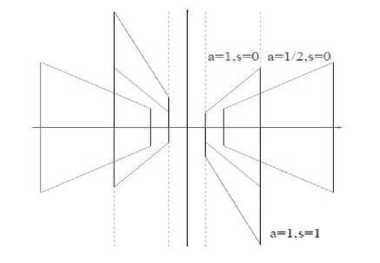
Fig.1. Frequency support of the shearlets p j,i,k for different values of a and s [8].

Where 1 1 e C ” (K) is a wavelet, and supp 1 1

II. Shearlets

The theory of composite wavelets provides an effective approach for combining geometry and multi-scale analysis by taking advantage of the classical theory of affine systems. In dimension n=2, the affine systems with composite dilations are defined as follows [8]

^aasow = {i j^k Cx) = MetA^ p⁽S ^l A ^j x -k):j, I e

Z, к e z}                    (2)

Where p e l2 (k2) is called composite wavelet. A,S are both 2 X 2 invertible matrix, and | det S| = 1, the elements of this system are called composite wavelet if AAs(p) forms a tight frame for l2(^2)^l< f,PLlik> I2 = llfll2

j,l,k

Let A denote the parabolic scaling matrix and S denote the shear matrix. For each a > 0 and s e R,

A = (i >=(0 S)

The size of frequency support of the shearlet is illustrated in Fig. 1 for some particular values of aand s. In [8], consider a = 4 , s = 1 ; where A = A₀ is the anisotropic dilation matrix and S = S₀ is the shear matrix, which are given by

A o = (0  0).S o = (0  1)

Fo V ^ = (ll)e R ² , ^ * 0, let ф ^{(0) (}О be given by

|- ¹ ,;т| ^u [-^Л] ; 1 2 e C” № and supp p 2

2 16        16 2

[-1, 1] .

[-

1 1 ] 2

2,2-*

.

This implies 1 ⁽⁰⁾ e C ” (K) and

In addition, we assume that

1 (0)

c

c

c

Zj20l11 (2-2M|2 = 1,H > 1/8

and for V j >  0

Z2i--127|p2(2jw-l)|2 = 1,|w|<1

Equation (3) and (4) imply that

£ Ц |i 0 Цл . S.)r ^ Ц |1m2 ² U|² |p 2 (2^j|-l)|² = 1

j>0 ,=-2i                         j>0 ,=-2i

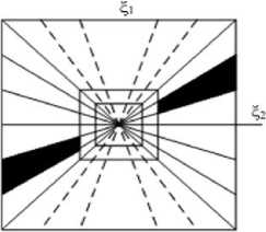
For any ⁽f_vf 2 ) e ^ 0 , where D 0 ={⁽f 1 ,f 2 ⁾ e R ² :|f 1 | >  1 ,|f₂| < 1}, the functions {p ⁽⁰⁾ (fA_o ^j S₍ - ¹ )} form a tiling of D₀. This is illustrated in Fig. 2(a). This property described above implies that the collection.

(a)

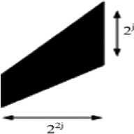
Fig.2. (a) The tiling of the frequency by the shearlets. (b) The size of the frequency support of a shearlet ^ j_-l-k [8].

(b)

{ 1 _j , _l , _k ⁽⁰⁾ (x)=22 p ⁽⁰⁾ (S 0 A ^j 0 X-k): j>0,-2 ^{j j} -1,keZ ² }

is a Parseval frame for 12 = (D0)v{f £ £2(T2) : supp f £ D0} based on the support of t and t2 can easily be observe that the functions t; k have frequency support, slфpф T С {(£,Ур£( -22 v22 4|U 2 2 4,22 jjk , |2 |<2 }

That is, each element $. z k is supported on a pair of trapezoids, of approximate size 22j×2j, oriented along lines of slope l2-j as shown in Figure 2 (b).

Similarly we can construct a Parseval frame for L² (D 1 ) ^v, where D 1 is the vertical cone,

D1={«1.b)eR2:|ti>V8|||<1}

Let Л = [0  4] and S = (}  1]

and t¹ ) be given by

t(1)(f) = ^С1)(|1Л2) = ^(М^ (I1)

where t and t2 are defined above. Then the collection [8]

t7(1)fc = 2~ t(1)(S1^x - fc): j> 0,-2j < 2j,fc £ X2

Is a Parseval frame for £ ² (D 1 ) ^v . Finally let t £ C ₀°° (T ² ) be chosen to satisfy

G(f) = |t(f)|2 + Rj + Pj = 1

Where

»t = I2l ■         •    (■ j>0 l=-2i

Pj = S7-aoS2=-1v| tC1)(fS1X^)|2^D1(f) = 1

for f £ T ²

where %D denotes the indicator function of the set D. This implies that t с [- ¹ , ¹ ] with |t| = 1 for f с [- ¹ , ¹ ] and the set {t(x - fc): fc £ X ² } is a Parseval frame for £2 ([- ^<1] ) . It is observed that, by the properties of t^(d),d = 0;1 , it follows that the function

G(f) = (I₁,|₂) is continuous and regular along the lines ¹² = ±1 (as well as for any other f £ T ² ) [8].

• III.    Basic Theory of Signal Sparse Representaion (SR)

SR is based on linear combination of a prototype signal from dictionary [12]. The following notation [12], considered f £ T ” be n real valued samples signal. The sparse representation theory the dictionary is formed on D £ T ^nxm , which contains m prototype signals. This dictionary D which determines the signal is sparse. In the dictionary D, there exists a linear combination of prototype signal and it shows Vx £ f, 3s £ R^T such that x ~ Ds, where s is sparse coefficients of x in D. It usually assumes that m > n, implying that the dictionary D is redundant and it follows Restricted Isometric Property (RIP) [12].This property solves the problem of reconstruction of signal with optimization problem to find the smallest possible number of nonzero components of s:

mins ||s||0 subject to | |Ds - x|| < £ (5)

This is called 1 0 -norm and ||s||₀ denoting the number of nonzero coefficients in sparses. This is an NP-hard problem. This problem can only be solved by systematically testing based on combinations of columns D.This problem is solved by greedy algorithms such as the basis pursuits (BP), matching pursuit (MP) and the orthogonal MP (OMP) algorithms [13].

• IV.    Sparse Repsentation for Image Fusion

The sparse representation (SR) handles an image in globally. But it cannot handle image fusion because it depends on the local information of source images. The source images are divided into small patches with fixed dictionary D to solve this problem. In addition, a sliding window technique and shift invariant are also important to image fusion for the sparse representation.

We consider that a source image I is divided into j small patches by size n x n as shown in Figure 3. It can be represented into lexicographically orders as a vector u . Then, V7 can express as u = ZT=1Sj(t)dt (6)

where j is the number of image patches and d_t is an atoms/prototype      from     D      and     D =

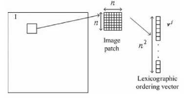
Fig.3. A source image patches and its lexicographic ordering vector.

The image patches of I are now rebuild into one matrix v. Then, v can be expressed as

			S 1 (1)	S2(1)   .	■ S>(1)1
v = [d1 ...	.dt...	.dr]	S 1 (2)	S2(2)   .	■ S > (2)	(7)
			51(T)	S2(T)	Sy(T).

Then the equation (7) can be expressed as

v = DS where S is a sparse matrix. Figure 4 represents the basic approach to fuse the image by sparse representation.

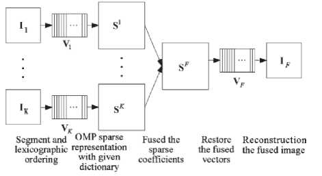
Fig.4. Proposed SR-based fusion method.

• V.    Image Denoising

Images are subject to noise which are captured and transferred from one destination to another. Noise can greatly affect the fusion result. So to make the fusion more effective this paper introduces thresholding to the respective coefficient values after taking the MST decomposition. We consider BayesShrink threshold which performs better than SureShrink in literature in terms of mean square error (MSE).

The BayesShrink threshold is given by [14]:

Wi) = |              (8)

an = median (|Detaifs|)/0.6745       (9)

The noise model of image x is considered as x = I + n and source image (I) and source noise (n) are assumed to be independent. Therefore the average noise (variance) and signal power can be calculated as,

0 2 = o i + о П                 (10)

where о ² is the variance of the observed signal о , is the noise density for source image. The output noise power of source image ст² is

^O i

Jmax(⁽o_s² - O_? ² ),0)

• VI.    Proposed Method

The proposed image fusion methodology contains the following five steps which are described below:

• A.    MST Decomposition: Apply MST on the two source images {I_A, I_B} to obtain their low-pass bands {L_A, L_B} and high -pass bands {H_A, H_B}.

• B.    Thresholding: Perform thresholding as obtained from Equation (7) on the low-pass and high-pass to remove the unnecessary coefficients from the decomposintion.

• C.    Low –pass fusion:

• i.    The image I is divided by appling sliding window technique to {I_A,I_B} into image patches of size Vn X Vn from upper left to lower right with a step length of pixels. We have also considered that there are T patches denoted as {f_A}^₁ and {P B }^₁ in L_A and L_B respectively.

• ii.    Rearrange {P A , P B } into column vectors and also rearrange {V A , V B } for each iteration by

VA = vA - VA. i

VB = vB - vB. 1

where 1 denotes one dimensional vector asn X 1 and V A and V B are average values of all elements in p and V B respectively.

• iii.    The sparse coefficients vectors {« A , « B } of {V ,V B }is calculated using OMP algorithm [13] by

«A = argmin H«H0 st ||VA - D«|2 < e «B = argmin H«H0 st |VB - Da|2 < e

Where D is the learned dictionary and e is tolerance of sparse value.

• iv.    Merge « A and « B with max-L1 rule to obtained the fused sparse vectors

  « F = ^{

  V

  
  

«A if ll«AH1 > ||«ВН1

«в       other-wise

The fused result of V X and V b is calculated by

VX=D«F + Vf1

Where the merged mean value   Vf is obtained by V = { V if «F = «B

( Vb  otherwise

The above iterative procedures for all the source image patch in {PA}^ and {РД}^ to obtained all the fused vectors

{p F } ;=i and{V F } ;=i .

vi. At the final steps the low-pass fused results denoted L_F . For each V F reshape it into a patch P F and then plug P F into its original position in L_f . As patches are overlapped, each pixel’s value in L_F is averaged over its accumulation times.

• D.    High-pass fusion: Apply threshold rule using Equation (7) for filter to ensure fused image contains source image. And then merge H_A and H_b to obtained H_F with  the popular  ‘max-absolute’  rule    each

coefficients of image A and B.

• E.    MST reconstruction: Perform the  corresponsing

inverse MST over L_F and H_F to reconstruct the final fused image I_F.

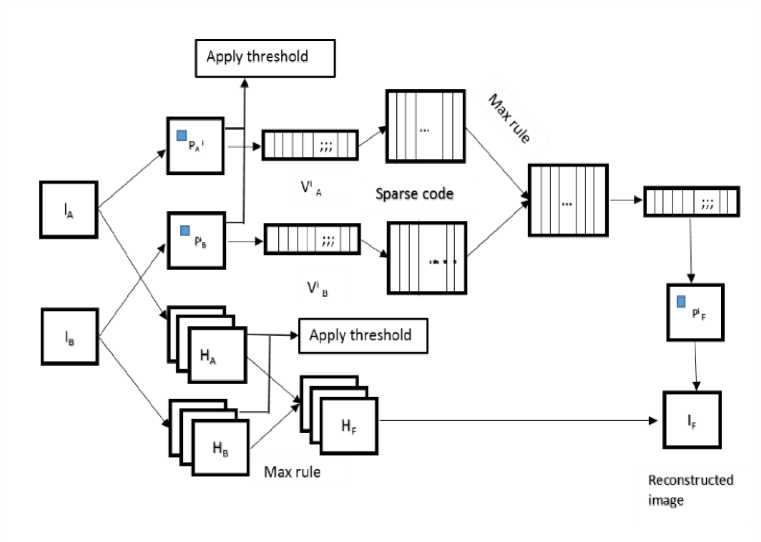
Fig.5. Block diagram of proposed method.

• VII.    Experiments and Analysis

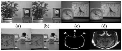
The source image pairs are taken from database [15 as shown in Figure 6,] and grouped of these images to apply proposed ST-SR method for image fusion and compare the results with other MST methods.

For dictionary process in image sparse presentation, we assign randomly values in dictionary D of size 64 X 256 from the image patches of training dataset image then sparse coding is done to get the sparse matrix of signal then K-SVD algorithm [11] has been run to update the dictionary. In simulation, we have estimated 100,000 of training data and 8x8 patches, and these patches are randomly sampled into image. In simulation, the dictionary size was set to 256 and the iteration number of K-SVD is fixed to 180.

(e)

(f)               (g)              (h)

Fig.6. Source images pair for experimental analysis[14].

For comparative studies, we have used different MST method and SR such as discrete wavelet transform with sparse representation (DWT-SR), dual-tree complex wavelet transform(DTCWT) and sparse representation (DTCWT-SR), curvelet transform and sparse representation (CT-SR), nonsubsampled contourlet transform (NSCT ) and sparse representation (NSCT-SR), non-subsampled shearlet transform (NSST) with sparse representation (NSST-SR).

Table 1. Performance mesurements of different image fusion method.

	Methods	Fig.4 (a)(b)	Fig.4 (c)(d)	Fig.4 (e)(f)	Fig.4 (g)(h)
SD	DWT-SR	52.2803	51.1927	47.2138	51.7858
	DTCWT-SR	51.8128	50.8592	46.9703	53.5718
	CT-SR	51.9511	50.8515	46.8730	54.4996
	NSCT-SR	52.1892	51.1708	47.2209	56.8796
	NSST-SR	52.9218	51.9778	47.9486	56.9551
MI	DWT-SR	6.4716	6.9422	7.0805	2.2327
	DTCWT-SR	6.9836	7.0816	7.4136	2.0315
	CT-SR	6.6547	7.0543	6.9303	1.9097
	NSCT-SR	6.9077	7.6748	7.5160	3.0118
	NSST-SR	6.9857	7.9168	7.9504	3.1877
EN	DWT-SR	7.4870	7.3228	7.1110	6.1926
	DTCWT-SR	7.4448	7.3318	7.0817	6.7317
	CT-SR	7.4642	7.3946	7.0999	6.8621
	NSCT-SR	7.4608	7.3292	7.0962	6.5892
	NSST-SR	7.6676	7.5513	7.4051	6.9054
SSIM	DWT-SR	0.8810	0.8907	0.9022	0.5449
	DTCWT-SR	0.8865	0.8938	0.9078	0.7004
	CT-SR	0.8862	0.8941	0.9070	0.6811
	NSCT-SR	0.8918	0.9015	0.9112	0.7637
	NSST-SR	0.8994	0.9098	0.9195	0.7692
AB/F	DWT-SR	0.6946	0.6810	0.7038	0.5773
	DTCWT-SR	0.7166	0.7102	0.7277	0.6334
	CT-SR	0.7023	0.6994	0.7069	0.5898
	NSCT-SR	0.7132	0.7216	0.7303	0.7368
	NSST-SR	0.7195	0.7271	0.7358	0.7394
Q G	DWT-SR	0.6874	0.6912	0.7171	0.5645
	DTCWT-SR	0.7071	0.7192	0.7368	0.6159
	CT-SR	0.6867	0.7087	0.7192	0.5713
	NSCT-SR	0.7025	0.7320	0.7400	0.7329
	NSST-SR	0.7096	0.7371	0.7473	0.7394

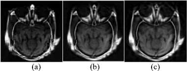
In this research work, five popular metrics have been used for evaluating the quality of a fused image [16] , which are Standard deviation (SD), Mutual information (MI), Entropy (EN), Standard similarity index metric (SSIM), Q^AB/F, the gradient based image fusion metric Q G represents in Table I. In Table I shows the proposed method such as NSST-SR is achieved the highest results in bold face mark for SD, MI, EN SSIM, Q^AB/F,Q_G than DWT-SR, DTCWT-SR, CT-SR, NSCT-SR. Also the fused image of NSST-SR shows good quality visual fused image in Figure 7 (e) for comparison with them.

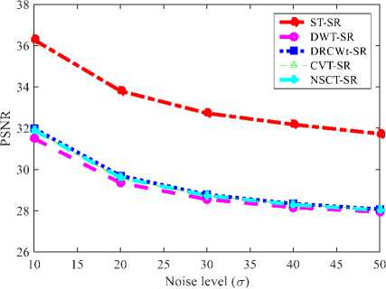
Table 2. Performance mesurements with different noise level for f different image fusion method.

Sigma(a)	Methods	PSNR
10	DWT-SR	31.4988
	DTCWT-SR	31.9889
	CT-SR	31.8623
	NSCT-SR	31.8978
	NSST-SR	36.2864
20	DWT-SR	29.3442
	DTCWT-SR	29.6937
	CT-SR	29.5617
	NSCT-SR	29.5967
	NSST-SR	33.8054
30	DWT-SR	28.5474
	DTCWT-SR	28.7777
	CT-SR	28.7332
	NSCT-SR	28.7283
	NSST-SR	32.7254
40	DWT-SR	28.1573
	DTCWT-SR	28.3370
	CT-SR	28.3004
	NSCT-SR	28.2909
	NSST-SR	32.1793
50	DWT-SR	27.9320
	DTCWT-SR	28.0779
	CT-SR	28.0589
	NSCT-SR	28.0208
	NSST-SR	31.7270

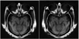
(d)                 (e)

Fig.7. Fused image of (a) DWT-SR, (b) DTCWT-SR, (c) CT-SR, (d)

NSCT-SR, (e) NSST-SR, for a = 0.

• VIII.    Conclusion

This paper work proposes a method for image fusion using MST and sparse representation. It gives us the result which overcomes the disadvantage introduced in MST and SR method individually. Training time for Dictionary in SR is relatively high. We use a dataset consisting different type of images and which contain about 40 images. For thresholding the image we have used bayesShrik thresholding which take the threshold value in different direction of image under certain transformation domain, which gives good threshold and results in a fused image which is noiseless in great measure. In the future, this model can be enhanced and cope with different efficient transformation domain which can take the geometry of image in better way. So it will be interesting to see how advancement is made in this approach.