Синтез фильтра координат угла прямой видимости на основе интерактивного многомодельного алгоритма оценки

1. Introduction. In the flight equipment, the target angular coordinate determination system is actually the tracking system that determines the target coordinate parameters. In an angle measuring device, the directional device generates signals that are proportional to the target tracking error according to the angle. This error in the vertical plane is determined by the angle Δφ d , between the signal balance direction of the antenna and the target direction [1-3]. Figure 1, O a and O t - the position of the control object (flight equipment) and the target in the non-rotation coordinate system X 0 O a Y 0 , attached to the flight equipment.

Fig. 1. Motion correlation between the flight equipment and the target

_{______}РОБ_{_}ОТОТ_{_}ЕХНИКА, АВТО_{_}МАТ_{_}ИЗАЦИЯ И С_{_}ИСТЕ_{_}МЫ УПРАВЛЕ_{_}НИЯ_{______} where: O a X oy - longitudinal axis of the flight equipment;

O a X a - the signal balance directional of the directional device;

ε d - angle of the line of sight to target in the inertial coordinate system X₀O_aY₀ ;

ϕ t - angle of the line of sight compared to the longitudinal axis of the flight equipment;

φ ad - the angle of rotation of the antenna compared to the longitudinal axis of the flight equipment (the directional angle of the antenna);

ϑ - flight equipment nodding angle;

O a O t - the flight equipment line of sight;

Δφ d - angle difference between the signal balance line and the line of sight.

The task of the problem determines the coordinates of the target angle: Generates angle ε d and ω d speed coordinate evaluations of the line of sight. On the current flight equipment control systems, the determination of ε d and ω d is done by the tracking one-loop angular coordinate determination system [4-7]. With this method, ε d and ω d are received using directly the signals from the antenna transmission system φ ad and from gyros measure the longitudinal axis angle ϑ . The evaluation error ε d and ω d of this method will be large, especially in the case of the maneuvering target, due to the fact that the antenna has large inertia [3, 811].

Based on the application of optimal control theory and optimal filtration theory, the target angle coordinate determination system on current flight equipment is built with the tracking multi-loop [12, 13]. This coordinate determination system has a smaller error than the tracking one-loop system, especially in the case of a maneuvering target, because ε d and ω d are evaluated by a separate tracking loop without using directly the ϕ ad signal as an evaluation signal [3, 14].

However, the tracking multi-loop coordinate determination system only takes into account the maneuvering target situation with specific values of maneuvering intensity ( σ ² j_t ) and maneuvering frequency ( α j ). That is, it remains unresolved for the class of the problem taking into account the diverse maneuverability in the reality of the target. Therefore, when the actual maneuvering of the target is not consistent with the hypothetical

_{____________}ROBOTICS, AUTO_{_}MATION AND C_{_}ONTROL SYSTE_{_}MS_{____________} model used to synthesize the coordinate system, the evaluation error ε d and ω d will increase.

Therefore, the task set out for the article: based on the tracking multi-loop coordinate determination system, building an algorithm to improve the accuracy of the target angle coordinates in maneuvering target conditions.

When applying optimal control theory and optimal filter theory, the problem of synthesizing systems to determine the target angle coordinates can be divided into two problems, namely:

The antenna control problem so that the signal balance line ( O a X a ) coincides with the direction of the line of sight ( O a O t ). This problem has been solved 3] or the optimal control technique [4, 9] can be used to synthesize the control law, so the article does not set out, but only applies the results when necessary.

The problem of evaluating the phase coordinate of the line of sight ε d , ω d takes into account the interaction of other parameters ( ϑ , ϕ ad ...) and the maneuvering of the target. This problem is solved by the article in the direction of synthesizing the adaptive system to improve the accuracy of the target angle coordinates in maneuvering target conditions.

The general method to improve the evaluation ε d , ω d in maneuverable target conditions is to use adaptive Kalman filtering techniques. Single-model adaptive filtering techniques perform the adaptation on the corrected phase or predictive of the Kalman filter algorithm [4, 15-18]. With these methods, the structure of the filter is relatively simple, however, the evaluation accuracy is not high and the maneuvering detection time is kept slow compared to the multi-model adaptive filtering techniques. In the multi-model adaptive filtration technique, with the assumption that the process follows one of the N known models, the evaluation accuracy is higher and the maneuvering detection delay is significantly reduced [3, 19-20].

• 2.    Synthesis of the line of sight angle coordinate filter.

  • 2.1.    Selection of different models for the interactive multi-model evaluation algorithm. The purpose of the line of sight angle coordinate filter is to evaluate the line of sight angle, line of sight angle speed and target normalization acceleration in order to provide the information required for the flying equipment guide law. With the optimal target angular coordinate system, this filter is designed with the Singer model with fixed parameters. Then, the model’s equation of state takes the form [3, 12]:

^d = ®d ,(1)

2D

®d=-—^d+D(j,-Jd),

j;=-«jj;+ $j,,(3)

where: D - relative distance between flight equipment and target;

• j , - normal acceleration of the target;

j_d - normal acceleration of the flight equipment; ^ j , - process noise of the model.

Based on this idea, the article adds 2 other models, characteristics for the small and large degree of maneuverability of the target. The model with constant velocity (CV model) and almost constant acceleration model (CA model) to build the interactive multi-model (IMM) evaluation algorithm for the line of sight angle coordinate filter. This choice is derived from the point of view, these 3 models are suitable for 3 different levels of maneuverability of the target.

Thus, the line of sight angle coordinate filter includes 3 linear Kalman filters running in parallel using 3 models, respectively, the CV model, Singer model and CA model. The final state evaluation is a combination of component filters with weighting on the exact probabilities of each model. As a result, the evaluation quality of the target phase coordinates is improved because the evaluation process has a redistribution of the probabilities of each model to suit the actual maneuverability of the target. The specific kinetics model to build these 3 filters is as follows:

• - The Kalman 1 filter uses a CV model for synthesis (Fig. 2). This model considers the target normalized acceleration as white noise j , = $ [5, 12]. In this case, the velocity and angle of the target orbital inclination ( 0 , )

• j                                                    .

are almost constant due to 0 = — (assuming the target velocity is constant).

• V ,

This model characterizes the degree of maneuverability of the smallest targets.

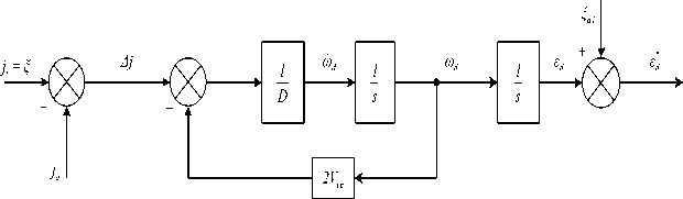
Fig. 2. CV model to synthesize the Kalman filter 1

The model’s equation of state takes the form:

I

ε_d= ω_d ,

2D112V 11

ω =- ω -j+ξ = ^tc ω -j+ξ .        (5)

d D d D d DD d D d D

Where: D ξ - line of sight angular acceleration noise, due to the uncertainty in the model CV causes, V tc =-D - target approach speed.

The vector form of the system of equations above:

Where: x 1

x 1 = ^Fmh1^X1^+Gmh1^U1⁺ w 1 .

εd ωd

- target phase coordinate state vector;

u 1 =j d - control signal;

F

F mh1

G mh1

mh1

2V tc

D

D

2 σ_a 2₁ D²

- state transition matrix of filter 1;

control matrix;

- covariance matrix of process noise.

The discrete model above with cycle T , the base matrix is calculated as follows:

Ф mh (t)=L - { (P l - F mh ) 1 } .

Inside: L -1 - inverse Laplace transformations, I - the unit matrix has dimensions consistent with F mh .

Replace the sampling cycle T with the variable t of the base matrix to get the transition matrix Φ mkh = Φ (T) .

The discrete form control matrix, received by the formula:

T

G^k mh = J Ф тк (t) .G mh dt •

The discrete form of the covariance matrix of the process noise:

T

Q kh = J Ф тк (Ж Ф (t)dt .

According to the above general formulas, the parameters of the CV model discrete form:

₁ D(β -1)

state transition matrix;

control matrix.

Ф mh1

G mh1

2V tc 0β

T D(β -1) 2V tc ^- 4V tc ²

1-β

The covariance matrix of the process noise discrete form as follows:

D(e2-1) D(e -1L. 3

-+T

Q mh₁ (1, 1) =

4V tc         V tc

4V C

Q mh , (1, ²)= Q    ^ 1) = f       1-1 ^ "  ,

I ^8V tc ^4V tc )

β ² -1 2

.

Q _{mh 1} (2, 2) = _{4V tc D} σ _{a 1}

2V tc T

Inside: β =e D , T - discrete cycle.

• σ a2₁ - process noise variance, which is characteristic of the maneuvering intensity.

• -    Filter Kalman 2 uses the Singer model (Fig. 3) to describe the target’s movement [5, 12-13]. This model characterizes the moderate maneuverability of the target, shown through the selection of two fixed parameters, maneuvering frequency α j and maneuvering intensity σ a2₁ . The kinetics of model 2 has the following form:

  

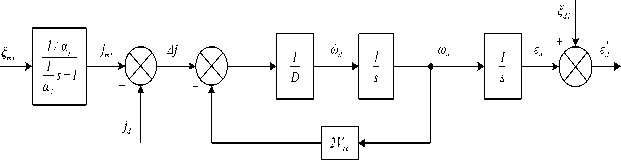
  Fig. 3. Singer model to synthesize the Kalman filter 2

  
  

1/α _j

In the above model, the input inertia stage () is the shaping s/α_j+1

filter. To create the target maneuvering style with constant intensity and the moment of maneuverability evenly distributed during flight time, the spectral density function of process noise ^ j has the form:

σ

2 ₌ ^j max2

a2

T f

.

Where: j max2 - maximized target normal acceleration, maneuverable; T f - flight time.

Equation of state of model 2 (Singer model).

The above equation is in vector form:

sd = ®d ,(7)

2V 11

ωd= Dtc ωd+Djt-Djd,(8)

jt=-αjjt+ξjt.(9)

The above equation is in vector form:

x 2 = ^Fmh2 x 2 ^{+ G}mh2 u 2 ⁺ w 2 ^.

Inside: x 2

εd ωd jtd

- target phase coordinate state vector;

F mh2

0	1	0
0	2V tc	1
	D	D
0	0	-αj

state transition matrix of filters 2;

G mh 2

control matrix;

D 0

Q mh2

2 σ a 2

- covariance matrix of process noise.

Similarly, we have the parameters of model 2 in discrete form:

1 De -1) 2Vt?	e aT 1 +        Dp       " а(2 Vte + Da) 2 V tc a + 2Vte (2V tc + Da)
Ф mh2 = 0 в	в -e -a 2V c +Da
0      0	e-T
[	J

mh2

T₊ D(1 - β) 2V tc 4V tc ²

1-β

2V tc

control matrix.

Covariance matrix of the process noise discrete form as follows: 2                                    32

(e^-αT-1)(^{8V tc} +4DV_tc)+T(D²α² +4DV_tcα+4V_tc²)-(β -1)( ^{D α} +2D²α)

Q (1,1)= α                                         Vtc mh2 ,                         4D2Vtc2α4 +16DVtc3α3 +16Vtc4α2

-^2Vtc2 (e^-2αT -1)+ ^{D 3 α 2 (β 2 -1)} + ^{4D 2 Vtcα} (e ^2V D ^{tc T -αT} α              4V_tc     2V_tc - Dα

4D2Vtc2α4 +16DVtc3α3 +16Vtc4α2

-1)

а2

a2

,

Q mh₂ (1,2)=Q mh₂ (2,1)=

2VtcT -αT                       2

D(e ^D    -1)-(β-1)(^{D α}+D)-(e ^-αT -1)(D+^{2V tc} )

2Vtc                     α

2D ² V_tcα ³ +8DV_tc ² α ² +8V_tc ³ α

₊ V tc (e ^-2αT -1) ₊ D ² α(β ² -1)

^а _____________ ^4V tc     . _ 2

2D ² V_tcα ³ +8DV_tc ² α ² +8V_tc ³ α ^a2

Q mh₂ (1,3) = Q mh₂ (3,1) =

(e^-αT-1)(D+ ^{2V tc})- ^{V tc (e -2αT -1)} αα

TF т

2V_tcT _-αT

₊ D²α(e ^D - 1)

2Vtc - Dα

4Vtc2α+2DVtcα2

• ° 2

Q mh₂ (2,2)=

2V_tcT _-αT

1-e ^-2αT ₊ D(β ² -1) 2D(e ^D -1)

2α      4Vtc - 2Vtc -Dα

D2α2+4DVtcα+4Vtc2

σ

a2 ^,

Q mh₂ (2,3)= Q mh₂ (3,2)=

Г     e^2T -1    + D(ee^-aT -1) )

( 2(Da² +2V tc a) ' 4V - D²a² J ° a²

-2αT

Q mh (3,3)= ^{1 e}   σ a ²

.

² 2α ²

• -    Filter 3 is synthesized based on the CA model (Fig.4). This model considers the target normal acceleration is almost constant (also known as the Jerk acceleration model is approximately equal to 0 ) [5, 12-13]. This model characterizes a high degree of maneuverability, when the target is to maneuver continuously at nearly constant acceleration.

  

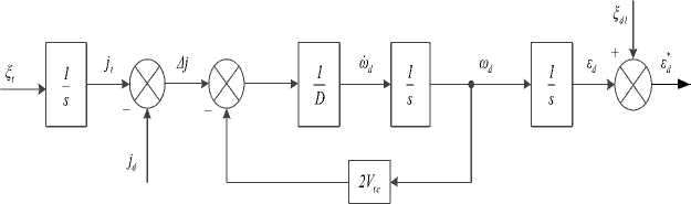
  Fig. 4. CA model for synthesis of Kalman filter 3

  Then, the model’s equation of state takes the form similar to (7), (8):

  
  

£ d ® d ,

2V 11 ω = ^tc ω +j- j , d D d D t D d

j t =ξ

In which, the input integral stage is the shaping filter. Similarly, to create the target maneuvering style with constant intensity and the moment of maneuverability evenly distributed during flight time, the spectral density function of process noise § ₅ has the form:

Where: j max3 - maximized target normal acceleration, maneuverable, T f - flight time.

Note, when designing each filter, the spectral density of the process noise in the Singer and CA models is different, due to the different maneuvering intensity.

Equation of state in vector form:

x 3 = ^Fmh3^X3^+Gmh3^U3⁺ w 3 .                     (13)

Inside: x 3

εd ωd

- Target phase coordinate state vector.

F , mh3

2V tc D

D

State transition matrix of filters 3.

G mh3

1 D 0

Control matrix.

Q mh3

0 0 0 Ст2

a3

Covariance matrix of process noise.

Switch to the discrete model, we have:

ф , mh3

₁ D(β -1)

2V tc

0β

D(β -1) T 4V tc ^{2 -} 2V tc β-1 2V tc

State transition matrix.

G mh3

Т D T+D(1-β)

2V tc 4V tc ²

1-β

2V tc 0

Control matrix.

Covariance matrix of the process noise discrete form as follows:

Q mh₃ (1,1) =

( D 3 (e² -1) + D²T

I 64V ' V-

DTI + DT² + T³ 1 ₂ 8V tC ⁺VC⁺V2V² ) ° a³

Q mh₃ (1,2)=Q mh₃ (2,1)=

f D² (в² -1) + DT DTP D²(e -1) ( 32V_t C ⁺V n -"VyT 16V²

1 „ 2

8V tC J a³

О                f D²(e-1) ^DT

Q mh 3 (^1,3) Q mh 3 (3,^) \    _QV3    — д 27 2

I ^8V tc      ^4V tc

2 T2 σ

4V tc ^J a³

Q mh₃ (2, 2) =

f DQ3²-1) D(P-1) +^_ 1 °2

( 16V tC      4V C     4V ^J a³

I D(e -1)   T 1

• ^Q mh 3 ^(2,3) Q mh ; !^3,2) I    ЛТ/2     ?Т/ I ^ a^? ,

• 2.2.    The algorithm to evaluate the coordinates of the line of sight angle with 3 different models. On the basis of the interactive multi-model filtering algorithm [15, 19-21], we have a general block diagram describing the evaluation algorithm of the line of sight angle coordinates shown in Figure 5.

к ^4V tc     ^2V tc )

Q mh₃ (3,3)=Tσ a ² ₃ ,

2VtcT where β =e D , T - discrete cycle.

The process of implementing the evaluation algorithm of the line of sight angle speed filter is as follows:

Step 1. Call p ij , ( i, j= 1,2,..., N ) – the probability of changing from the model i at time (k - 1) to the model j at time k . This probability is constant throughout the evaluation process. We choose the model transfer probability matrix as follows:

0,9995 0,0001 0,0004

П - 0,0004 0,9995 0,0001

0,0001 0,0004 0,9995

In which, model 1 is CV, model 2 is Singer and model 3 is CA.

Call μ j (0) - model probability at the time of initialization. In the beginning, the true probabilities of the 3 models are equal, so:

μ CV (0) = μ SINGER (0) = μ CA (0) = 3 .

Step 2. Calculate the mixing probability, that is, the appearance probability of the i th model at time (k - 1) with the j th model condition at time k .

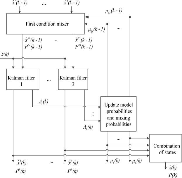
Fig. 5. Block diagram of line of sight angle coordinate filter with 3 component

Kalman filters: p^(k-1) is defined as:

цЛ](к-1)

=   p j p i (k-1); with i,j = 1,2,3 ;

cj c j = £ Pi jPi (k -1); with j = 1,2,3 .

i=1

Step 3. Mix the first condition for the j't* filter:

Input status, after mixing:

55^0j(k-1) = У x^-1)^-1); With j = 1,2,3 ;           (15)

correlation of input errors, after mixing:

5c^0j(k-1) = У x ⁱkk-1)^_u(k-1); With j = 1,2,3 ;            (16)

-т 1

P ^J(k-1)=У^ j k-1){ P (k-1)+ [ X (k-1)- 5i?( k-1) ][ X (k-1)- 5 ?' (k-1) ] } X ⁰(k-1)

i=1

= У х X(k-1)^ t _!jj(k-1); With j=1,2,3.

i=1

Due to the fact that the state vector size in the CV model is 2, and the Singer model and the CA model are 3, we need to solve the problem of mixing three models with different state vector sizes. In [15, 22-24] has proposed several ways to solve the problem. Here, we simply choose that when mixing for the CV model (model with smaller state space size), we only mix the corresponding state components in the Singer and CA model, ignoring the states remaining. When mixing for Singer and CA models (the model with larger state space size), we consider the missing state components in the CV model to zero.

Step 4. Perform evaluation algorithm of each component filter, with the first conditions, is mixed:

Evaluate the a priori of each filter:

5c^- (k) = Ф ^ 5c ^j(k-1) + G^J _k ii ^j(k-1) ;                      (18)

inside: Ф-', - state transition matrix corresponding to the model j ; G^J _k -control matrix corresponding to the model j .

Calculate the a priori error correlation matrix of each filter:

P ^-(k) = Ф ( P ^0j(k-1)[Фи^т + Q k (k-1) .

Calculate the Kalman amplification matrix:

K (k) = P ^-(k) H T (k)x [ H j (k) P ^-(k) H T (k) + R k (k) ] ^-1 .          (19)

Inside, R^J_k(k) = a • - variance of observed channel noise. Here, we consider the variance of the measurement noise in all three models to be equal.

With the CV model, the Kalman amplification coefficient is only 2:

k¹*- ^P"*_. , ¹ p ; ; (k)+a •

K 1 (k)= P^, . 2      P 1 (k) + a •

The Singer and CA models are respectively:

K(k)= ^P -^{1 (k)} ₂ , P^J , (k) + a • ’

K^J₂(k) = -^PPJk-^ ,

•^w p ;; (k)+a • ’

K₃(k) = —^P(k^ .

P?.(k) + a •

Evaluate the posterior state (after measurement update) of each filter:

x^J (k) = 5c ^{- j} (k) + K^J (k) [ z (k) - H^J (k) 5c ^{- j} (k) ] .

The posterior correlation matrix of each filter:

P ^J (k) = [ I - K ^J (k) H ^j(kc) ] P ^-(k) .

Step 5. Calculate the logical function for the filter j"' :

Л_- (k) = N [ z (k); z^j [ k | k -1 ; 5c ^0J(k-1\k-1) ] , S^j [ k, P ^0J(k-1\k-1) ]] . (21) It means, Л _j(k) = N [ e^J(k);0;S^J(k) ] , inside:

e j (k) = z (k) - H ^j x " ^J (k-1) ,

S , (k) = H , [ Ф ^ P ^0j (k -1)[ Ф f + Q k J H J + R ,

1            1 T

Л ) = ^^х ^ехР1^(k)S_j'(k)e_j(k)) ,

V 2^{n8 (k)}     2

Л , (k) =

, ¹ exp(- — ¹— e 2 (k)) . 2n8sk^ ^И 2S j (k) ^iV"

Step 6. Updated j"' model probabilities:

k j ^(k)=~ ^Л j ^(k)^c j ;

c = ^ Л j (kjc j - normalized constants.

j=i

Step 7. Combination of evaluation states and error correlation matrix after updating the correct probabilities of each model.

Combination of evaluation states:

P j Xk)^¹ ^(k)^c j

Combination of error correlation:

P (k) = ^^^^ P j (k) { P^j (k) + [ x^j (k) - 5c(k) ] [. x ^j (k) - x (k) ] ^T } .

• 3.    Simulation results and analysis. To survey the quality of the tracking multi-loop target angle coordinate system using the interactive multi-model filtering algorithm, we will simulate the angular coordinate system with different maneuvering styles of the target in the horizontal plane (Fig. 6). Then, compare with the quality of the optimal angular

• 3.1.    In the case of a ladder type maneuvering target:

coordinate system (with fixed parameters based on Singer model) according to the criteria of mean square error (MSE).

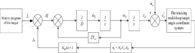
Fig. 6. Diagrams simulation of the target angle coordinates system in the ideal flight equipment control loop

• -    The target’s initial position: x_t(0) = 40(km) ; y_t(0) = 0(km) .

• -    The flight equipment initial position: x(0) = 0(km),y(0) = 0(km) .

• -    The target flies in at velocity: 350 (m/ s) .

• -    The flight equipment velocity: 1000(m/s) .

• -    The target’s initial trajectory tilt angle: 9 _t =0° .

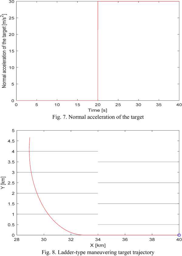
• -    The normal acceleration of the target:

  30 (m / s² )

  
  

  when <20s

  when t> 20 s

  
  
  
  

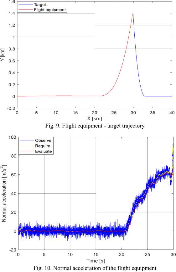
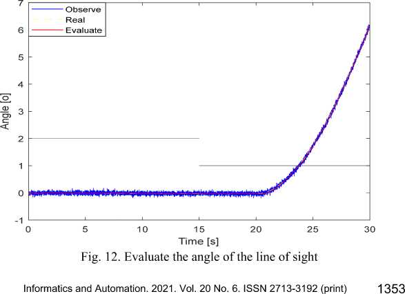
With this model, initially, the target has evenly straight movement. After 20 seconds, the target suddenly maneuvers continuously with constant normal acceleration 30 (m / s 2 ) . Thus, the target has a change from a non-maneuverable model to maneuverability with constant normal acceleration. This motion model has uncertainty in maneuvering moment and maneuvering intensity. The simulation results of the target angle coordinate system for the case of ladder-type maneuvering targets are as follows (Fig. 7, 8). Figures 10-17 reflect other features of the analyzed process.

After 20 seconds of steady straight movement, the maneuvering target with constant normal acceleration. This causes the required normal acceleration of the small missile at an early stage (before 20 seconds), then increases continuously until the meeting point. However, the flight equipment normal acceleration filter still gives a good evaluation.

Time [s]

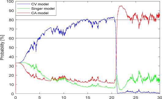
Fig. 11. The graph shows the correct probabilities of the model

Figure 11 shows that from 0 to 20 seconds, the CV model dominates, but after about 22 seconds (the transition time of the IMM algorithm is about 2 seconds), the probability of the CA model is clearly dominant compared to the other 2 models. This trend continues to maintain in the remaining maneuverable time of the target. This evaluation result of the algorithm reflects quite correctly with the actual maneuvering of the target.

The results of evaluating the target phase coordinate for the case of ladder-type maneuvering target are as follows:

ISSN 2713-3206 (online)

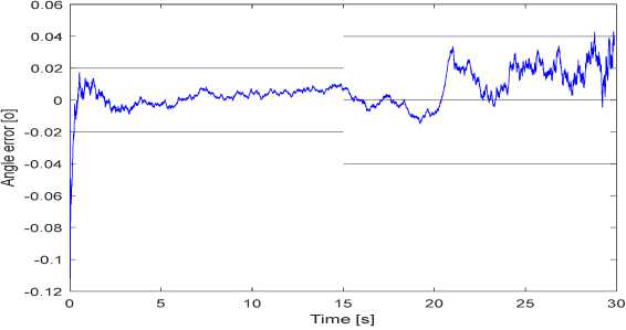
Fig. 13. Evaluation error of the line of sight angle

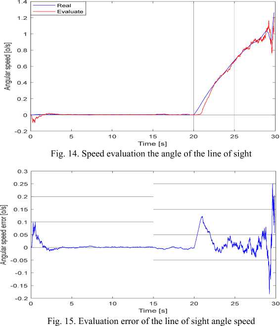
The simulation results show that in all 3 states: the angle of view, the angle of view and the normal acceleration of the target, the IMM evaluation algorithm gives a greater error at the time the target starts to maneuver (model change time). But right after that, the clinging error is smaller. Compare the quality of the IMM filter algorithm with the optimal filter algorithm after 100 Monte-Carlo runs:

Time [s]

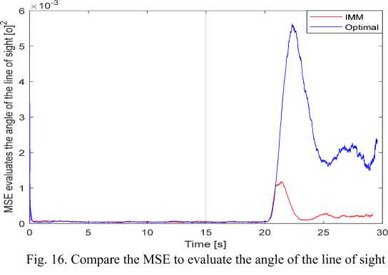
Fig. 17. Compare the MSE to evaluate the angular speed of the line of sight

Before the maneuvering target time (20s), the evaluation quality of the two algorithms was equivalent (the evaluation error of the optimal filtering algorithm was trivial smaller). But after 20 seconds, there is the

_{______}РОБ_{_}ОТОТ_{_}ЕХНИКА, АВТО_{_}МАТ_{_}ИЗАЦИЯ И С_{_}ИСТЕ_{_}МЫ УПРАВЛЕ_{_}НИЯ_{______} difference in evaluation quality. Detail:

• -    With the line of sight angle, the evaluation error of the IMM algorithm at the time of maneuvering model transfer (change) is MSE(e_d) ~ 1,2.10'³ [(o) ] , also the optimal filtering is MSE(e_d) ~ 2,5.10'³ [(o) ] . Then, at the stable tracking stage, the optimal filter algorithm for error is MSE(e_d ) ~ 0,85.10 - [(o) ] , the IMM algorithm is MSE(e_d ) « 0,25.10 - [(o) ] .

• -    With the angular speed of the line of sight, the evaluation error of the IMM algorithm at the time of maneuvering model transfer is MSE( rn _d ) ~ 0,012 [(o / s)²] ,     also the optimal filtering is

MSE ( ® _d ) ~ 0,015 [(o / s)² ] . At the stable tracking stage, the optimal filter algorithm for error is MSE( & _d ) ~ 0,004 [(o / s)² ] , the IMM algorithm is MSE( ® _d ) ~ 0,001 [(o/ s) ] .

• -    With the target normal acceleration, at the time of maneuvering model transfer, both algorithms give large evaluation errors MSE(j_t) ~ 900 [(m / s² )² ] . At the stable tracking stage, the optimal filter algorithm for error is MSE(j_t) ~ 220 [(m / s²) ] , while the IMM filter gives a significantly smaller error with MSE(j_t) ~ 10 [(m / s² )² ] .

• 3.2.    In the case, the maneuvering target according to the Singer model. The parameters of the initial position, the velocity of the flight equipment and the target remain the same as before, but differ in the target normal acceleration.

Obviously, when the maneuvering target with constant acceleration, the evaluation quality of the target angular coordinate system using the IMM filter algorithm improved when compared to the optimal filter algorithm.

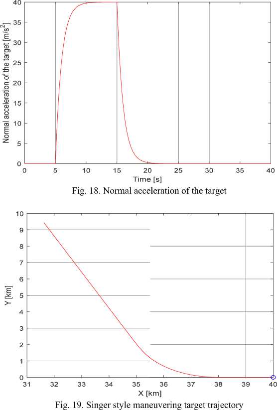
The target normal acceleration is generated from the following kinematic model:

Where: a j =1 (1 / s) , T - discrete integral cycle, u - control signal or maneuver command.

0 when t < 5s u = < 40 ■ ajt (m / s2)

when t < 15 s .

when t > 15s

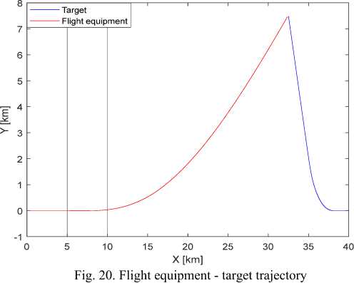
With this model, initially, the target has evenly straight movement. After 5 seconds, the target begins to maneuver in a Singer model with a command acceleration is 40(m / s²) . After 15 seconds, the target reverted to its non-maneuver style. Thus, this motion model has uncertainty in maneuvering moment, maneuvering time and maneuvering intensity.

The simulation results of the target angle coordinate system for the maneuvering target case according to Singer model are as follows:

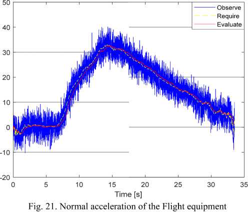
When the target starts to maneuver, the normal acceleration requires an increase and when the target changes to the non-maneuver model, the required normalized acceleration of flight equipment tends to decrease to 0 .

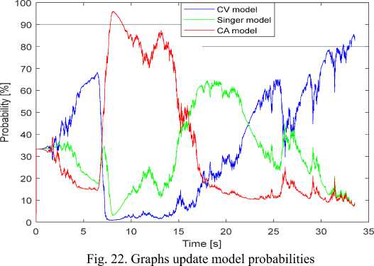
Obviously, when the target has evenly straight movement in the first 5 seconds, the CV model dominates over the other 2 models. In the time of the maneuvering target (5 ÷ 15s), the CA and Singer models dominate again, in which the weight of the CA model is greater because the target maneuvering command, in this case, is quite large ( 40m / s 2 ) makes the CA model fit with more practical. And when the target ends maneuver time, the correct probability belongs to the CV model.

Time [s]

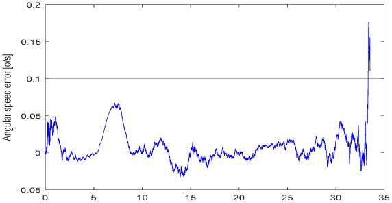
Fig. 26. Evaluation error the angular speed of the line of sight

Similar to the case of a maneuvering target with constant normal acceleration, in this case, all 3 target phase coordinates have a larger evaluation error at the time of model transfer (from non-maneuver to maneuver and on the contrary), but then IMM filter algorithm gives smaller evaluation error.

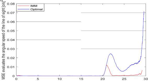
Comparing the quality of the IMM filter algorithm with the optimal filtration algorithm after 100 runs of Monte-Carlo for the case of Singer style maneuvering target gives the following results:

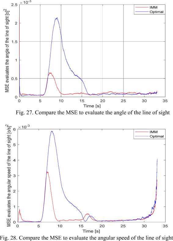
MSE simulation results show that in the non-maneuver target stages (before 5 seconds and after 15 seconds), the evaluation quality of the line of sight angle coordinate filter when using the IMM filter algorithm is slightly worse when compared with the optimal filtering algorithm. However, at the maneuvering target stage (5 ÷15 seconds), the evaluation error of the IMM algorithm is significantly smaller. Detail:

• -    At the moment the target starts to maneuver, for the optimal filtering algorithm is MSE(ε_d ) ≈ 2,2.10^-3 (o)² , MSE(ω_d ) ≈ 6.10^-3 (o / s)² , MSE(j t ) ≈ 1000 (m / s 2 ) 2 ; also for the IMM filtering algorithm is MSE(ε_d ) ≈ 0,6.10^-3(o)² , MSE(ω_d) ≈ 3,2.10^-3(o / s)² , MSE(j_t) ≈ 850(m/s²)² .

• -    At the stable tracking stage, for the optimal filtering algorithm is MSE(ε_d ) ≈ 0,7.10^-3(o)² , MSE(ω_d) ≈ 1,7.10^-3(o / s)² , MSE(j_t) ≈ 600(m/s²)² ; also for the IMM filtering algorithm is MSE(ε d ) ≈ 0,1.10 -3 (o) 2 , MSE(ω_d ) ≈ 0,15×10^-3(o/s)² , MSE(j_t) ≈ 30 (m/s²)² .

• 4.    Conclusions. The article has synthesized the line of sight angle coordinates filter between the flight equipment and the target using the interactive multi-model adaptive filter technique. The suboptimal target angle coordinate tracking system is constructed from individual filters and combined with an antenna control system to create a multi-loop target angle coordinate system. Obviously, the target’s maneuvering directly influences the evaluation filter the line of sight angle coordinate. So, in order to synthesize the target angle coordinate determination system with high accuracy in the maneuvering target conditions, just need to improve the line of sight angle coordinate evaluation filter, keeping the other filters.

The simulation results of the tracking multi-loop target angle coordinate system show that, when comparing the quality of the line of sight angle coordinate filter using the IMM filter algorithm based on the MSE criteria, the evaluation error is smaller than the optimal filtering algorithm under different maneuvering target conditions. Here, the change of the target maneuvering styles while the flight equipment approaches the target, highlighting the advantages and reliability of the interactive multimodel evaluation algorithm. The advantage is that during the evaluation process, the algorithm will always update the closest approximate model to the actual motion of the target, resulting in a combination of state evolution from the component filters giving results more precisely, the optimal filter has a fixed parameter. Of course, the more models that are taken into account when designing the line of sight angle coordinate filter, the higher the adaptability of the filter to target maneuverability, but we need to consider the cost of calculation and real-time response of the electronic computer on board.