SNR Improvement by Photon Noise Filtering in Ocean Color Monitor Satellite Images

Published Online February 2016 in MECS

ISRO’s Oceansat-2 satellite carried three payloads, Ocean Color Monitor (OCM), Ku-band Pencil Beam Scatterometer and Radio Occultation Sounder for Atmosphere (ROSA). The payloads of this mission are tailored for making measurements of the physical and the biological oceanographic parameters.

OCM-2 has eight multi-spectral bands in VNIR region. With IGFOV (Instantaneous Geometric Field of View) of 360X236m it covers swath of 1420 Km. At sea reference radiance, it provides PSNR ~300 with 12-bit digitization.

In any electro-optical imaging system, SNR (Signal to Noise Ratio) defines quality of measurement within detection range [1]. Definition of SNR is as follows.

Signal

N°isephoton)+(NoiseDark) +(NoiseReadout) +(NoiseElectronics)

fAnscombe ( X )=2√ +

SNR       ⁼

Signal Radiance NoiseRadiance

For this specifically converted Gaussian noise removal, among many algorithms, which exist in the open literature, the sigma filter [10] is probably one of the simplest de-noising methods. Due to its simplicity, this filter represents a good choice for implementation.

However, the edge preservation performance of the sigma filter is not good, especially for small image details with variance close to the variance of the additive noise. In order to improve the detail preservation of the sigma filter, other more sophisticated approaches are proposed. For instance, proposed fuzzy filter [11] uses some fuzzy estimates of the local derivative to perform directional filtering of the image. Although it provides good filtering performances, this approach have the disadvantage of relative high complexity. Another alternative, hybrid sigma filter [12] is also proposed for speckle noise reduction. The hybrid sigma filter, however, does not address the problem of additive noise reduction which is the focus of our work.

This paper provides a new photon noise filtering which combines Anscombe transformation [6] and modified Sigma filter [13] for photon noise reduction in images. In our proposed method the input image is first decomposed in four components and a sigma filter is applied separately on each of them. The output image is then reconstructed from the four filtered components.

The paper is organized as follows. In section 2, the modified sigma filter is described. In section 3, the denoising algorithm is summarized. Section 4 provides results.

• II.    Modified Sigma Filter

First, we briefly review the standard sigma filter for additive noise [10] and outline its advantages and disadvantages. We assume the following model for the input image:

"У ( i.) ) = 4 i.) ) + n( i, ) ) (4)

‘y(i, j)’ is the observed image, ‘x(i, j)’ is the original clean image and ‘n(i, j)’ is a zero mean Gaussian distributed additive noise.

The main idea of the sigma filter is based on the fact that for a Gaussian distributed variable with mean μ and variance σ ² , a percentage of 95.5% of its samples lies inside the range [μ-2σ, μ+2σ]. Applying this observation to the model from (4), for every pixel y(i, j) from the observed image, a local average is computed on those neighboring pixels (in window of M × M) that are inside the interval [y(i, j) - 2σ, y(i, j)+2σ]. Corresponding pixel of the output image f(i, j) is replaced with this local average. A block diagram for de-noising based on sigma filter is depicted in Fig. 1.

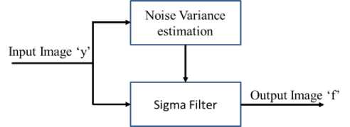
Fig.1. Denoising based on Sigma Filter

The input image is first passed through the noise estimation module and the estimated noise variance is then used in the sigma filter for de-noising. It is well known, that small details of the input image are not well preserved by the sigma filter. This is due to the fact that on the regions from the input image that have variance close to the noise variance almost all pixels from the local M × M window are used in the average process. For instance when the estimated noise variance is larger than the real noise level the blurring effect is evident. An immediate solution is to decrease the length of the selection range to [y(i, j)-kσ, y(i, j)+k σ] with k < 2. This modification reduces also the filtering capabilities of the sigma filter in smooth areas of the input image.

Taking into account these observations, we introduce a simple modification that improves the performances of the sigma filter for regions of the input image that contain small details.

The block diagram of our proposed Sigma filter is depicted in Fig. 2, where the blocks denoted as HPV and HPH perform a high-pass filtering on the vertical and respectively horizontal directions. Noise estimation is performed by the blocks denoted as NE and the sigma filters are represented by the blocks Sigma.

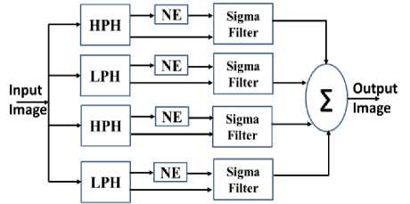
Fig.2. Proposed Modified Sigma Filter based denoising technique

Four component decomposition can be performed as follows:

YLPH (i, j) = [I(i, j) + I(i, j+1)]/2(7)

YHPH (i, j) = [I(i, j) - I(i, j+1)]/2(8)

YLPV (i, j) = [I(i, j) + I(i+1, j)]/2(9)

YHPV (i, j) = [I(i, j) - I(i+1, j)]/2(10)

Computation of these differences transforms the horizontal monotonically increasing/decreasing regions of the input image into constant regions [14]. Moreover this operation also preserves the edges from the input image. Transformation of the monotonic regions into constant regions makes the simple averaging, performed by the sigma filter, a better model. The coefficient 1/2 is introduced to preserve the dynamic range. It does not influence the filtering accuracy and it can be discarded at this point.

If Y(i, j) has noise variance σ _n ² then noise variance of four components can be written as [r14]:

^aLP H = ^aHP Н = ^aLP V = ^aHPV = "у        ⁽¹¹⁾

Reverse computation can be done by:

Y(i, j) = [Y _LPH (i, j) + Y _HPH (i, j) + Y _LPV (i, j) + Y _HPV (i, j)]/2                          (12)

Std - dev =

¹1.1 У V [Im age ( i , j ) - Mean ] 2 m n i = o j = o

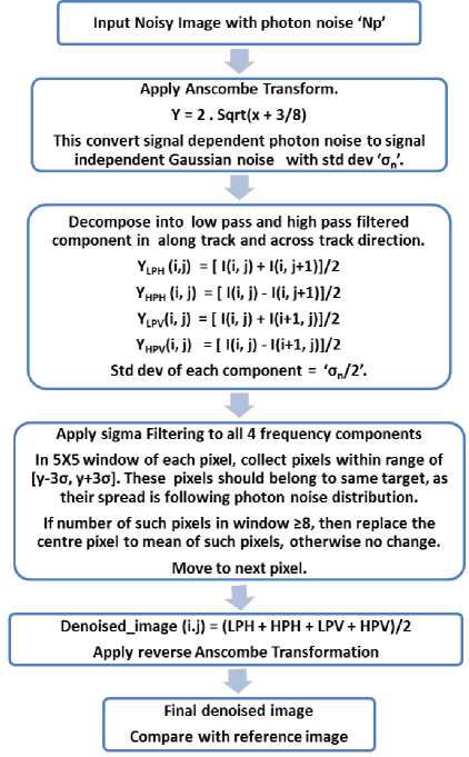
III. Proposed Denoising Algorithm

Typical flow chart of proposed denoising algorithm is given below.

|     |   m - 1 n - 2

L ine _ complexity =—.---- VV I Im age ( i , j ) - Im age ( i , j + 1)1

m n - 1 i = 0 j = 0

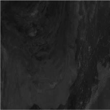
Fig.3. Simulation Image-set 1 (1000X1000)

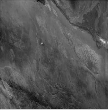
Fig.4. Simulation Image-set 2 (1000X1000)

• IV. Simulation Image-sets

  As no ground truth data is available, radio-metrically corrected 12-bit OCM-B1 images with PSNR=1000 is considered as reference image-set. Pixel wise Poisson distributed noise (with PSNR = 256) is added to this image and noise filter (as mentioned in previous section) is applied. Filtered image is compared with reference image to evaluated denoising performance.

Fig. 3-7 shows these image sets. Respective histograms are shown in Fig. 8-12. Table 1 shows parameters of simulation image-sets. For these parameters, equations are shown below [15].

m - 1 n - 1

Mean =   . VV Im age ( i , j )          ⁽¹³⁾

• m n i= 0 и

  

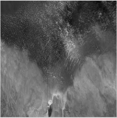
  Fig.5. Simulation Image-set 3 (1000X1000)

  
  
  

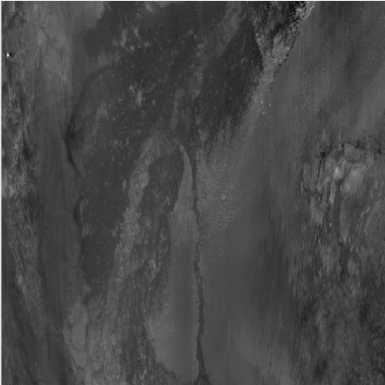
  Fig.6. Simulation Image-set 4 (1000X1000)

  
  
  

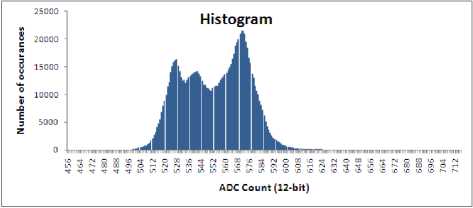
  Fig.10. Histogram of Simulation Image-set 3

  
  
  

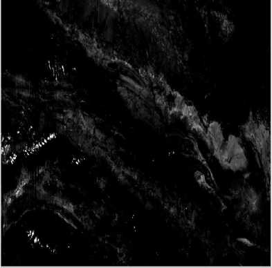
  Fig.7. Simulation Image-set 5 (1000X1000)

  
  
  

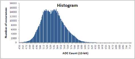
  Fig.11. Histogram of Simulation Image-set 4

  
  
  

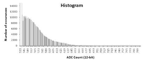
  Fig.12. Histogram of Simulation Image-set 5

  
  
  

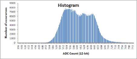
  Fig.8. Histogram of Simulation Image-set 1

  
  

  Table 1. Image parameters of Simulation image-sets

  	Imagesize	Mean	Std-dev	Row complexity
  Image-1		604	46	8
  Image-2		550	27	4.4
  Image-3		553	21	3.5
  Image-4		554	25	6.2
  Image-5		552	26	4.9

  
  
  

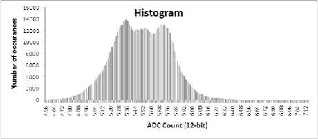
  Fig.9. Histogram of Simulation Image-set 2

  
  

  V. Simulation Results

  Noisy images with PSNR= 250 are filtered by denoising approach explained in previous sections. This section highlights results. Table-2 provide RMSE results comparison between noisy and denoised image.

  
  

  Table 2. RMSE results with noisy images of PSNR = 250

  	RMSE Noisy Image	RMSE Denoised Image	Mismatch (%) Denoised
  Image-1	6.3	4.6	0.83
  Image-2	6.0	3.6	0.87
  Image-3	6.0	3.1	0.87
  Image-4	6.9	4.1	0.88
  Image-5	6.0	3.6	0.87

  
  

  For computing equation is used.

  
  

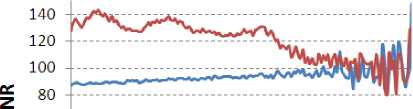
SNR at every count ‘S’, following

SNR ( S ) = 20log ₁₀

S                          =. hist ( S )

I         £ ^{( [} S - denoised ⁽ i , j ^{) ] 2} + ^[ Noise system ^{( S ) ]} 2 )

V ¹ , j ( ref _ image,. ¹ , j ) e ' ^S ')

Figure 13-17 provide SNR improvement analysis [15] in Image-set1 to 5. Lesser SNR improvement is also because of less number of occurrence of that particular count (refer histogram in Fig 8-12). This may be noted that proposed algorithm provides more improvement with images of lower contrast.

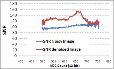
Fig.13. SNR improvement in Image-set1

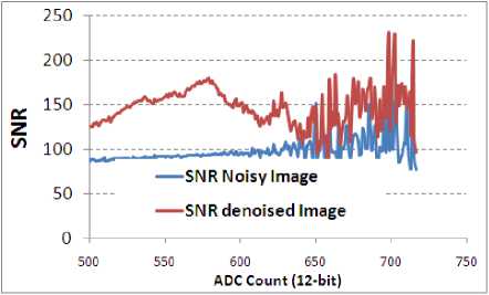
Fig.14. SNR improvement in Image-set2

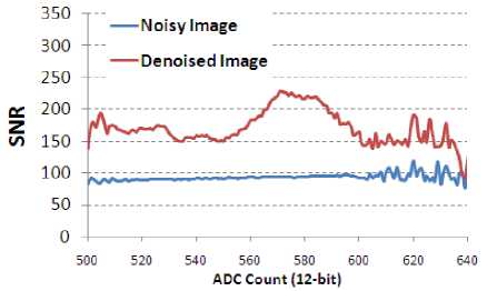
Fig.15. SNR improvement in Image-set3

^ so 4

40 ----- ---Noisy Image

20 ----- ---Denoised Image

0 ।                             ।                             ।                             ।                             ।                             ।                             ।                             ।

500    520    540    560    580    600    620    640

ADC Count (12-bit)

Fig.16. SNR improvement in Image-set4

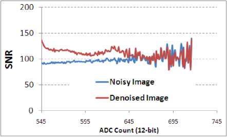
Fig.17. SNR improvement in Image-set5

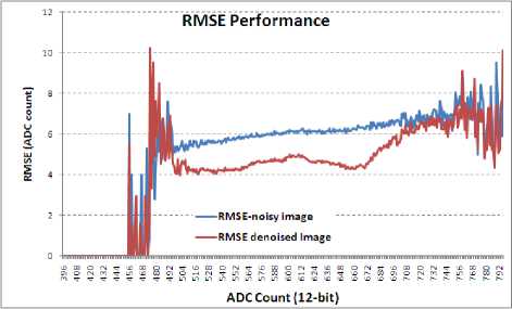
Fig.18. RMSE analysis of Image-set1

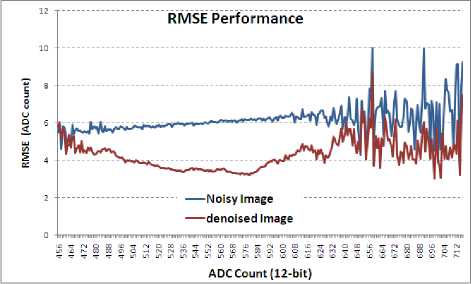
Fig.19. RMSE analysis of Image-set2

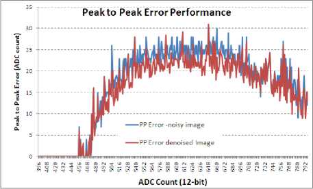
Fig.20. Peak to Peak error analysis of Image-set1

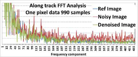
Fig.21. FFT Analysis for along track data in Image-set1

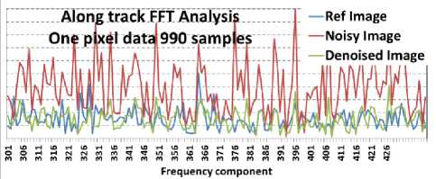
Fig.22. FFT Analysis for along track data in Image-set1 (zoomed form of Fig. 21)

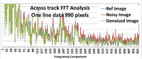
Fig.23. FFT Analysis for across track data in Image-set1

• VI. Conclusion

Proposed photon noise filtering techniques reduces photon noise significantly. Simulation results shows 20 to 50% reduction in RMSE. Count-wise SNR analysis is carried out. Significant SNR improvement SNR improvement is achieved. FFT analysis shows reduction of amplitude of high frequency noise components. Proposed technique is of low complexity and suitable for implementation. Simulation results can be further verified on more number of images before final implementation.

Acknowledgment

We gratefully acknowledge the constant encouragement and guidance received from Shri DRM Samudraiah- Prof. Satish Dhawan Scientist, Shri Saji A Kuriakose– DD-SEDA and Shri A. S. Kiran Kumar-Director SAC. We are thankful to our colleagues of Payload Checkout Electronics Group for providing the images.