Software Implementation of CCSDS Recommended Hyperspectral Lossless Image Compression

Published Online March 2015 in MECS

Hyperspectral images provide information in large number of narrow, contiguous spectral bands. It is used for mineralogy, pollution monitoring, atmospheric study, astronomy and many more. Hyperspectral images have three dimensions. Two of which are of Spatial and third one is spectral. Each scene is captured on all the spectral bands. Therefore each image has more information than traditional images. The very high amounts of data produced by such imagery and the bandwidth constraints of satellites, requires the use of on-board image compression techniques. There are various methods of compression as described in [6, 15]. There are methods for Hyperspectral image compression like Low Complexity (LOCO-I) [8], Two Dimensional Context Adaptive Lossless Inter-band Compression (2D-CALIC) [9] , Three Dimensional Context Adaptive Lossless Interband Compression (3D-CALIC) [10], Modified Context Adaptive Lossless Inter-band Compression M-CALIC [11] Look-Up Tables (LUT) [12] (using a single LUT), Locally Averaged Inter-band Scaling (LAIS)-LUT [13] and LAIS-Quantized LUT (LAIS-QLUT) [14] (LAIS-LUT and LAIS-QLUT using two LUTs). Various Hardware implementations are shown in references [16, 17]. Main technique of all image compression algorithms is to remove redundancy. Hyperspectral images have spectral redundancy other than spatial redundancy. Hyperspectral images differ from traditional images in that they require specific coding techniques that exploit its spectral redundancy to achieve competitive compression performance.

The Consultative Committee for Space Data Systems (CCSDS) composed of the world’s major space agencies, is a multi-national forum for the development of communications and data systems standards for spaceflight [1]. The Multi-spectral and Hyperspectral Data Compression (MHDC)[7] working group of the CCSDS has developed the CCSDS-123.0-B-1 standard [2], which is based on the fast lossless (FL) compression algorithm and intended for onboard lossless coding of multi- and hyperspectral imagery. Multispectral images have narrow bands over a discrete spectral range, and having less number of bands than hyperspectral images. This recommended standard achieves state-of-the-art compression performance on images captured by a wide variety of hyperspectral/multispectral sensors. It’s advantage of low computational complexity facilitates implementation in onboard resource constrained scenarios.

In this Paper, Section II introduces MATLAB implementation of algorithm in detail with various stages. Section III presents test results. The conclusion is given in Section IV.

• II.    Matlab implementation of algorithm

Compressor

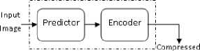
Recovered

I mage1"

Image

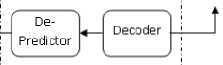
De-co moressor

Fig. 1. Basic block diagram of the scheme

Compressor has two functional units: a predictor and an encoder. De-compressor does reverse process of compression. De-compression is required to get original image. De-compressor has two functional units: a decoder and a de-predictor.

• A.    Predictor

  

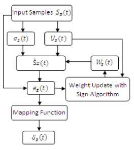
  Fig. 2. Flow chart for Predictor

  
  

Predictor uses an adaptive linear prediction method to predict the value of each image sample. S z,y,x or S z (t) is current sample value having D number of bits. Here, x & y represents spatial coordinates, z represents spectral dimension and index t is defined as, t = y.N _x + x. Where, N _x represents image width. Prediction of sample S _z,y,x is Ŝ _z,y,x is derived by computing ‘local sum’ σ _z (t) and ‘local difference’ U _z (t) with weight vector W _z (t). Weight vector can be initialised by default and custom method[2]. In default initialization method, Weight vector is initialized by particular default value.A weight initialization vector in custom based initialization method might be selected based on instrument characteristics or training data, or might be selected based on a weight vector from a previous compressed images. Therefore we have selected default initialization method of weight vector.These parameters are dependent on the values of nearby samples in the current spectral band and P previous (i.e., lower-indexed) spectral bands. The user-specified parameter P (range: 0 ≤ P ≤ 15) determines the number of previous spectral bands used for prediction. The prediction residual e z,y,x is the difference between the predicted Ŝ z,y,x and actual S z,y,x sample values. The prediction residual is then mapped to an unsigned integer δ z,y,x that can be represented using the same number of D bits as the input data sample. These mapped prediction residuals is the predictor output. Flow chart of Predictor is shown graphically in fig. 2.

• B.    Encoder

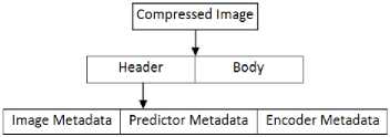
Fig. 3. Compressed image structure

• >    Sample adaptive encoder

The original FL (Fast Lossless) algorithm uses an adaptive coding approach using Golomb-Power-of-2(GPO2) codes. Under the sample-adaptive entropy coding option, each mapped prediction residual δz (t) shall be encoded using a variable-length binary codeword. The selection of the code used to encode δz (t) is based on the values of the adaptive code selection statistics which consist of an accumulator and a counter that are adaptively updated during the encoding process. Initial counter (γ ₀ ) and accumulator (K) value is in the range of 1 ≤ γ ₀ ≤8 and 0 ≤ K ≤ D– 2 respectively. Here, we have taken γ ₀ =1 and K=5. The interval at which the counter and the accumulator are rescaled is controlled by the user-defined rescaling counter size parameter γ^*, which shall be an integer in the range: max {4, γ 0 +1} ≤ γ^*≤ 9.

• >    Block adaptive encoder

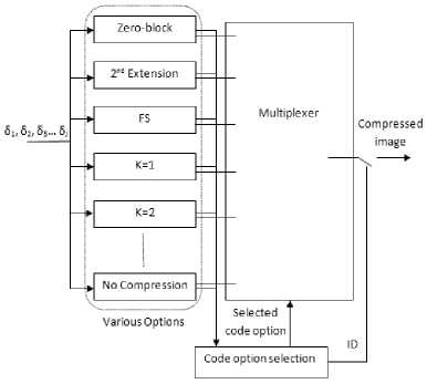
Fig. 4. Block adaptive encoder

The block-adaptive coder, which also makes use of GPO2 codes, is the Rice coding algorithm as formalized in the CCSDS 121.0-B-2 standard [3]. Block adaptive coder encodes samples on group of samples called Block. The block size parameter J shall be equal to 8, 16, 32, or 64. Shorter values of the block length parameter J allow faster adaptation to changing source statistics. Longer block lengths often offer improved overall compression effectiveness because of reduced overhead. So, we have taken J=16.The reference sample interval parameter, r shall be a positive integer not larger than 4096.We have taken r=1024. Packetized telemetry is used to limit error propagation as described in reference [3]. The Rice algorithm uses a set of variable-length codes options like Zero-block, 2nd extension, Fundamental Sequence, Nocompression as shown in fig. 4 to achieve higher compression Each code is nearly optimal for a particular geometrically distributed source. Variable-length codes compress data by assigning shorter codeword to symbols that are expected to occur with higher frequency. By using several different codes and transmitting the code identifier, algorithm can adapt to sources from low entropy (more compressible) to high entropy (less compressible).

• C.    Decoder

• >    Sample adaptive decoder

Decoding for sample adaptive encoder is simply reversing the procedure of encoding. By calculating number of zeros and ones, we can calculate accumulator and counter value. From that we can calculate the mapped prediction residual <5z(t).

• >    Block adaptive decoder

Block adaptive encoder encodes the block with some ID bits. From that ID bits, we get to know about which option is selected for encoding at the decoder side. Decoding for block adaptive encoding options like zeroblock, second-extension and no-compression are briefly given in CCSDS 120.0-G-3 informational report [4].

• D.    De-predictor

De-predictor consists of postprocessor and de-predictor stage. De-predictor stage reconstructs the original samples from previous samples similar to the approach used in DPCM decoding. First Sample S _z (1) of each band is not coded. Second sample S _z (2) is decoded from first sample S _z (1) value and second sample mapped prediction residual δ _z (t). Similarly all sample values are calculated. The postprocessor reverses the mapping function & gives the predicted value S z (t) .

• III.    Verification

  CCSDS 123.0-B-1 recommended standard is developed in MATLAB 2012a. Four hyperspectral images taken from different sensors are applied to algorithm and verified.

Dataset-1: It is from AVIRIS (Airborne Visible/Infrared Imaging Spectrometer) calibrated radiance images which is most widely used images for benchmarking hyperspectral image compression algorithms[5].It has solar reflected spectrum from 400 nm to 2500 nm at 10 nm intervals.We have taken 16-bit Yellowstone calibrated scene 11 raw image of size 512 lines x 677 samples x 224 bands.Three adjacent bands of Yellowstone calibrated scene 11 cropped images of size 256*256 are shown in fig. 10.

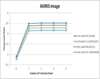
Fig. 5. Compression Ratio vs Number of Prediction band for Dataset1

AVIRIS

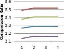
Fig. 5(A). Compression Ratio vs Number of Prediction band for Dataset1

Dataset-2: It is from Hyperion Level 0 images which are provided by the EO-1 Mission, NASA [5].Hyperion imager has 400 - 2400 nm spectral range and 10 nm spectral resolution. We have taken 12-bit Lake Monona un-calibrated image having width 256 and height 3176 with 242 spectral channels. In the files provided by the hyperion imager, each sample is stored as a 2-byte unsigned integer in little-endian byte order, samples arranged in Band Interleaved by Pixel order. Three adjacent bands of Lake Monona scene cropped images of size 256*256 are shown in fig. 11.

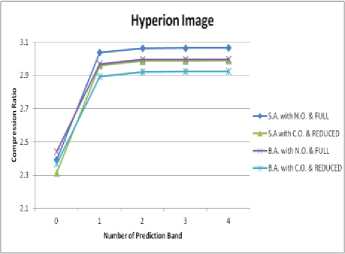
Fig. 6. Compression Ratio vs Number of Prediction band for Dataset2

Dataset-3: It is AHYSI (Airborne Hyper Spectral Imager) chandryan-1(CH-1) experimental data having 64 band data with 512 lines. Each line has 256 samples. AHYSI data are in RAW format. It is in band sequential Order. Its bands are in 400-950 nm range with 8.6 nm spectral resolution. Three adjacent bands of dataset-3 are shown in fig. 12.

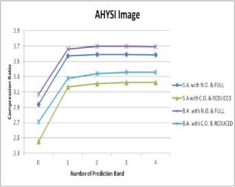
Fig. 7. Compression Ratio vs Number of Prediction band for Dataset3

Dataset-4:    It is FTIS (Fourier Transform

ImagingSpectrometer) data which is an experimental data. FTIS data is 32 bands data with 288 lines. Each line has 336 samples. FTIS data are in TEXT format. It is in band sequential Order. Its bands are in visible range. Three adjacent bands of dataset-4 are shown in fig. 13.

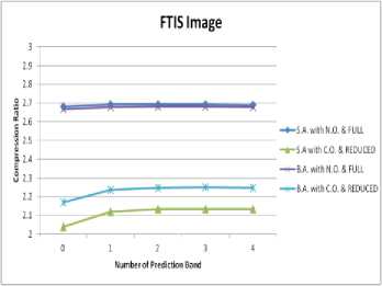
Fig. 8. Compression Ratio vs Number of Prediction band for Dataset4

Table 1. Compression ratio for four images

En. Type	Local Sum Type	Pre. Mode	Pre. band	AVIRIS (Dataset-1)	Hyperio n (Dataset-2)	CH-1 (Dataset-3)	FTIS (Dataset-4)
S.A.	N.O.	Full	0	1.9200	2.3930	2.9400	2.6802
			1	3.4910	3.0375	3.5736	2.6910
			2	3.5181	3.0629	3.5898	2.6932
			3	3.5178	3.0641	3.5887	2.6919
			4	3.5164	3.0650	3.5873	2.6904
	C.O	Reduce d	0	1.7958	2.3154	2.4562	2.0386
			1	3.2652	2.9595	3.1665	2.1209
			2	3.2875	2.9859	3.2110	2.1331
			3	3.2868	2.9882	3.2242	2.1345
			4	3.2857	2.9891	3.2248	2.1334
B.A.	N.O.	Full	0	1.8989	2.4415	3.0704	2.6657
			1	3.3768	2.9688	3.6610	2.6783
			2	3.4045	2.9944	3.6959	2.6813
			3	3.4046	2.9956	3.6955	2.6802
			4	3.4033	2.9966	3.6942	2.6788
	C.O	Reduce d	0	1.7768	2.3673	2.7092	2.1694
			1	3.1365	2.8921	3.2772	2.2376
			2	3.1605	2.9203	3.3395	2.2492
			3	3.1603	2.9227	3.3558	2.2503
			4	3.1593	2.9236	3.3572	2.2492

En. Type =Encoder Type, Pre. =Prediction, S.A.=Sample Adaptive, B.A.=Block Adaptive, N.O.=Neighborhood Oriented, C.O. =Column Oriented

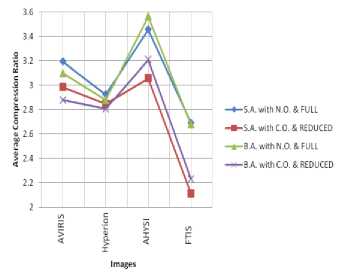
Fig. 9. Average Compression Ratio for different images

Compression Ratio of four images with Neighbour Oriented and Column Oriented prediction mode and with Full and Reduced Prediction mode for both encoding method is shown in Table I for four datasets. From fig. 9, it can be seen that Compression ratio for Full prediction mode in combination with Neighbourhood Oriented is better than for reduced prediction mode in combination with Column Oriented for all images. Average compression ratio is average of compression ratios for p=0 to 4. From figure 9, it can be seen that AHYSI image has more compression ratio. Spectral resolution is difference between two consecutive wavelengths of sensors.The finer the spectral resolution, more the spectral redundancy. AHYSI image has more spectral redundancy because of fine spectral resolution of only 8.6 nm which is less than other three.

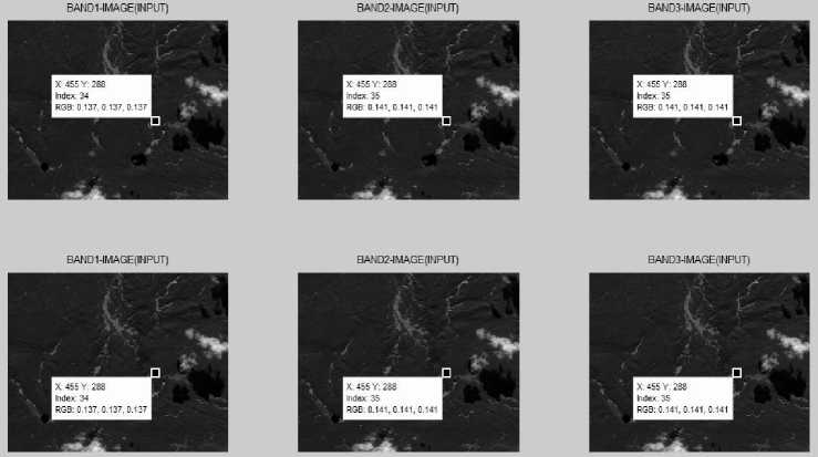
Fig. 10. Inputs and Output of dataset1

Fig. 11. Inputs and Output of dataset2

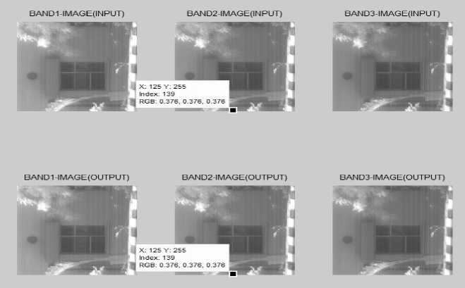
Fig. 12. Inputs and Output of dataset3

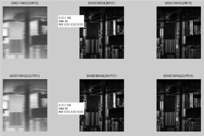
Fig. 13. Inputs and Output of dataset4

• IV.    Conclusion

We have successfully implemented CCSDS recommended algorithm for hyperspectral and multispectral compression namely CCSDS 123.0-B-1 in MATLAB. The developed algorithm is verified by applying 4 sets of real HySI data from different payloads namely AVIRIS, Hyperion, AHySI and FTIS as input to the system and reconstructing the images pixel by pixel. Results show that Compression ratio is about 2 to 3 for previous prediction bands of P>=2 and MSE is Zero. Compression system can be useful to reduce higher memory requirement constraint or higher bandwidth requirement constraint or both constraints of Hyperspectral imager payloads of space satellites. MSE is equal to zero shows that algorithm is fully lossless. Hyperspectral image compression system hardware can be implemented in FPGA with low complexity.