Soil surface subsidence time series modeling of an area with Aridisols and Vertisols complex using surveying and drone imagery in Central Iran

Soil surface subsidence and crack formation on the plains with clay soils was reported in Yazd, Iran (Akhavan Ghalibaf, 2008). Overexploitation of groundwater resources could be a reason for soil surface subsidence (Bhattarai et al., 2017). Soil surface subsidence is oftenly caused by three distinct water-related processes: 1) compression (compaction or consolidation) of bedded layers of clay and silt within the aquifer system; 2) drainage and oxidation of organic soils; and 3) dissolution and collapse of soluble materials (Bazargan, Esmaeil, 2010). Some of the serious effects of soil surface subsidence includes change of gradient along water conveyance canals, gas and oil pipes, damage to roads and bridges. Also collapse of aquifers after soil surface subsidence results from decreased groundwater volume (Aminihosseini, 1993; Pacheco-Martínez, 2013). Understanding and detecting soil surface subsidence at initial stages is important to prevent land use damages (Fulton, 2014). One of the most important issues in soil surface subsidence management is to predict the processes of soil surface subsidence changes over time. In addition, the prediction of soil surface subsidence during groundwater extraction by warning systems allows officials to reduce the damage caused by its further occurrence and to take special measures in advance to control it. In some places on the clayey soils of Yazd, where depression and giant cracks have occurred on the lands, calcareous-silicon concretions (lime dolls features) can also be seen with dimensions from a few centimeters to 20 centimeters and the core reasons of this phenomena are groundwater extraction and the presence of clay and amorphous silicas in the soil (Akhavan Ghal-ibaf, 2008). Skempton (1953) and Bjerrum (1954) found active clays and made the designation for the clay activity in the soil. In order to predict changes in soil surface, various models have been used which among stochastic statistical models are often used extensively in various aspects and contexts, including the time series model or the BoxJackins model, which is widely used in hydrology and climatology science for modeling and predicting data (Aghelpour et al., 2016). Chen et al. (2015) investigated spatial-temporal evolution patterns of soil surface subsidence with different situation of space utilization in Beijing, China, during 7 years with multi-temporal InSAR method incorporating both PS and SB approaches. The results showed that the soil surface subsidence had developed very quickly and the regional soil surface subsidence rate was not only related to the groundwater exploitation, but also related to dynamic load and underground space utilization. Ty et al. (2021) studied spatio-temporal variations in groundwater levels and the impact on soil surface subsidence in CanTho, Vietnam, using groundwater level assessment from 2000 to 2018. The results indicated significant downward trends of groundwater level and the average subsidence rate of 4.28 cm per year was observed. Su et al. (2021) investigated vertical movement rate of soil surface subsidence from 1960 to 2010 (six decades) using Global Navigation Satellite System (GNSS) data in north China plain and obtained the average vertical movement of soil surface subsidence of 31.13 mm per year. Li et al. (2021) modeled spatio-temporal soil surface subsidence with Permanent Scatterer-Interferometric Synthetic Aperture Radar (PS-InSAR) method. They realized that groundwater level variation is not a unique factor of soil surface subsidence in the study area and the spatiotemporal characteristics of soil surface subsidence under multiple variables can be used to predict soil surface subsidence due to groundwater level variations. Chu et al. (2021) estimated soil surface subsidence with spatio-temporal data fusion and found that the subsidence varies with time and space. Azarakhsh et al. (2022) predicted soil surface subsidence over time from 2014–2017 with Sentiel-1 time series in Teh-ran-Shahriar plain. The results showed that the soil surface subsidence is active and some factor combination that related to soil surface subsidence displacement including precipitation, ground water table change and depth to water table along with the distance from faults and thickness of fine-grained soil layers (clay and silt). The aim of this study is to predict height variations of soil surface subsidence and soil cracks in the course of time using direct surveying data and finally test- ing model with drone imagery data to increase land stability with monitoring in time and revealing hazard zones of land depressions.

MATERIALS AND METHODS

Study area

The study area located in the east of Yazd on the clayey desert soils in Khavidak district, geographical coordination: 40R, 31°50'35'' to 31°50'45'' N and 54°28'30'' to 54°28'45'' E (Figure 1).

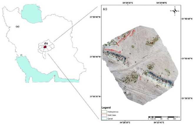
Fig. 1. Geographic location of the study area ( a ) Iran, ( b ) Yazd city and ( c ) East of Yazd city. Green lines: Vegetation cover ( Haloxylon sp. ). Red lines: Soil crack. Blue lines: Qanat.

The selected area for intensive observation limited to about 7 hectares. The common feature in the study area was microrelieves on the lands and two types of surface soil crack (longitudinal and polygonal). This phenomenon was adjacent to Yazd, the famous historical city in Central Iran, which was registered in UNESCO (UNESCO, 2017). For wind erosion control, species of desert resistant plants like Haloxy- lon sp. were planted as vegetation cover with the climate of extra arid and cold.

The air photos from years 1967 to 2020 are presented in Figure 2. According to the air photos, in 1967 the area was buried under sand dunes, but after 24 years due to protection of the area from further wind depositions the clayey soil surface has appeared. Last image by drone after 29 years shows less plant covers ( Holloxylon sp. ) after decreasing water table lower than 100 meters from soil surface.

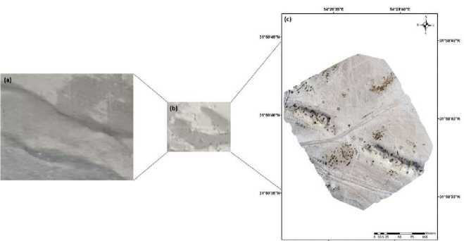
Fig. 2. The pictures from left to right show: air photos ( a ) 1967 (Scale: 1 : 20 000), ( b ) 1991 (Scale: 1 : 40 000), and drone imagery ( c ) 2020 (Scale: 1 : 1 000).

The study area consists of the old pluvial flood clayey plain of Quaternary geological age. These depositions were surrounded with depositions of younger piedmont plain. The origin of depositions consists of Triassic geological period of Mesozoic with Nayband formation to conglomerates of Eocene geological period of Tertiary (Hajmollaali, Majidifard, 2000).

Survey of research area and soil sampling

Soil samples were taken from the soil profile horizons in the dynamic positions where land surface was unstable with upward and downward movements and soil cracks. Then the soil samples were collected from the horizons on sample profile for complementary analyses, including the first depth of 0–20 cm as A horizon, second depth of 20–100 cm as B and Bqk horizon in depth of 100–200 cm and the last soil sample were taken from the depth more than 200 to 300 cm as C horizon. The usual soil chemical properties were analyzed in saturated paste extracts by traditional methods such as electrical conductivity (EC) as salinity index, and sodium adsorption ratio (SAR) as alkalinity index. The soil physical property as Soil texture measurements were performed using hydrometer (Gee, Bauder, 1986). Table 1 presents Activity Designation of clay that change from low-active to active.

Table 1. Designation of clay with regard to activity according to Bjerrum (1954)

Activity Designation
0 < CA ≤ 0.75	low-active
0.75 < CA ≤ 1.4	normal
1.4 < CA ≤ ∞	active

Skempton (1953) studied the relation between plasticity index and clay content in clay. Rankka et al. (2004) revealed that this relation was designated the clay activity (CA) and defined as Equation 1:

CA = PI/C,

where PI (% plasticity index) = LL (% liquid limit) – PL (% plastic limit), C = % clay content.

COLE (Coefficient of Linear Extensibility) was measured via the spherical soil in the plastic limit and calculated using Equation 2 as follows (Golden, 2014):

COLE = ^V _V ^m _d - 1,

where: Vm is spherical volume of wet soil and Vd is spherical volume of dry soil.

Soil surface subsidence and soil crack height variations measurements at specific times

In order to study the height variations (Height or Z) within the study area, 4 concrete stations are placed indicated as S1, S2, S3 and S4 in the 4 corners for grid the area to survey height variations and 100 pines were hit as index points by random systematic sampling (Shal-abh, 2018) in the study area. Then to determine micro movement of soil surface subsidence and soil crack (Z) was used Leveling method with a level detector with an accuracy of ± 3 mm and plate level (Werner, 1968). Leveling calculations were performed by the height of level and the height of all index points is determined from stations S1 and S3. Then in the following periods the measurements had been repeated with the same accuracy and sensitivity and compared with the same points of previous and first periods. The process of height variations of index points in soil surface subsidence and soil crack by measurements was modeled with the result of overlap of three-dimensional topographic layers at different times. Measurements were carried out in wet and dry months of year in December 2014, January 2015, February 2015, March 2015, May 2015, August 2015 and November 2015 and December 2015, across 12 months except April 2015, September 2015 and October 2015 because it did not show any difference from the March 2015 because clays against dryness and wetting lead to surface dynamics. Finally, the measure changes were drawn with the Kriging simple method (Arc GIS 10.6 software). The prediction model of height variations created with EViews 10 software. Finally, for monitoring and testing prediction dynamic model (Height, Z) in the study area was used Phantom 4 drone for high resolution imagery with 20 mega pixel camera from 50 meters flying altitude with the resolution of 5 cm for the pixel sizes (Figure 3).

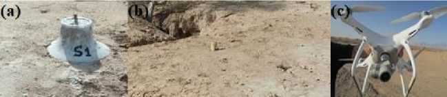
Fig. 3. A concrete station as standard point ( a ), index points ( b ) for measuring by level detector and Phantom 4 drone for high resolution imagery ( c ).

After taking the desired images, the necessary processing was done to generate dense point clouds using Agisoft photo scan software (Jebur et al., 2018). In this step, matching points between images are overlapped, the camera position is estimated for each image, and an initial and sparse point cloud model was created. Aligning the images were done to identify the points in each image and perform the matching process with the same point in two or more images (Anurogo et al., 2017). For the actual image production stage, the highest accuracy is used in Align Photo. Dense point cloud model was done after leveling and testing the accuracy of ground control points. The final output of this process was a 3D structure that also provides information about the relative positions of the camera and the relative distances between the camera and the object (Dellaert et al., 2000). The next steps include meshing and digital elevation model (DEM) construction, respectively. Creating the mesh was the stage of the 3D or polygonal model, which is one of the main outputs of Agisoft aerial image processing, which is used for 3D modeling for creating DEM with the accuracy of 3 mm.

Research methods

In statistical science and signal processing, the time series model also known as Box Jenkins model, is a model commonly used to measure data sorted by time. The observed time series can be considered as the result of a stochastic process. The simplest model that can be considered to simulate this time series is related to the process in which events occur at separate times and at regular intervals and each of them is independent of the other values (Box, Jenkins, 1976). Famous time series models included Auto Regressive (AR), Moving Average (MA), Auto Regressive Moving Average (ARMA) and Auto Regressive Inte- grated Moving Average (ARIMA). In this research due to the instability of the data of height variations over time, the ARMA model was suitable to predict the time series.

Auto Regressive Moving Average model (ARMA)

The first sub-model, ARMA (autoregressive moving average), has two components: an autoregressive (AR) component and a moving average (MA) component. The autoregression (p) and moving average (q) parameters define the model. The AR component of an ARMA model predicts a variable’s value based on its own lagged (i. e. prior) values. The MA component of the model predicts a variable’s value as a linear combination of past error terms. The Box-Jenkins method is used to evaluate the parameters of the model by using the calculation of the Akaike, Schwarz and Hannan-Quinn info criterion (Shahriari et al., 2022). The ARMA model can be written as Equation 3:

(1 - ϕ1 B - … - ϕp B^p) Y t = c + (1 - θ 1 B - … - θq B^q) α t ,        (3)

where B denotes the Box-Jenkins backshift operator (B^pY t = Y (t-p) ), ϕ and θ represent the vectors of the autoregressive and moving average parameters, respectively, c – refers to the model intercept, α t is a series of independent random errors with zero mean and variance σ².

In this study by using the surveying data, one-year height variations (2014 – 2015) up to 2020 was predicted using Eviews 10 software (Agung, 2011) and for testing model, the modeled data was compared with drone data obtained from year 2020.

RESULTS AND DISCUSSION

Soil physical, mechanical and chemical properties in typical sample profile in cracked lands

According to the amount of clay, silt and sand in Table 2, soil texture of A and B horizons are silty clay, in dolls (Bqk) are loam and in C horizon is sandy clay. The soil electrical conductivity (EC) showed high salinity in soil profile. The index of pH and SAR show more alkalinity in soil surface (horizon A). The amorphous silica content in the soil horizon A is higher than in other soil horizons.

Table 2. Soil texture and soil chemical properties of the study area

Soil horizon	Depth (cm)	Clay (%)	Silt (%)	Sand (%)	Soil texture	EC (1:5, soil/water extract,) (dS/m)	pH (1:1, soil/water suspension)	Amorphous silicas in soil (%)	SAR
A	0–20	42	48	10	silty clay	3.50	9.0	7.0	17.00
B	20–100	41	44	15	silty clay	3	8.4	5.0	12.00
Bqk	100–200	12	47	41	loam	2.20	7.8	1.0	10.50
C	200–300	44	9	47	sandy clay	2.80	7.2	0.5	11.70

The results of COLE and CA in the study area are provided in Table 3. Soils with more than 0.03 COLE in B horizon could have the criteria of smectite minerals for surface dynamic and Gilgai features according to Dixon and Weed (1992). CA data shows that the clay roles for land surface dynamics could not be strong. These soils, according to Golden (2014), were classified as vertisols order in US soil taxonomy. Also because of aridic soil moisture regime known as Tor-rert suborder and related to the petrocalcic horizon (Bqk) and existence of duripans were classified in subgroup of Leptic Calcitorrerts.

Table 3. The amount of COLE and CA

Soil horizon	COLE	CA
A	0.02	0.32 (Low activity)
B	0.14	0.28 (Low activity)
Bqk	-	0.44 (Low activity)
C	0.03	0.13 (Low activity)

Micro relief monitoring in study area

• Figure 4    presents topographic map in the study area. Red lines are soil cracks of two types: polygonal and longitudinal. According to the figure below, the area demonstrated variability including micro anticline and micro syncline type. The base of study was the same as previous research in the area has presented by Amin et al. (2019).

The amounts of height variations using surveying data registered on the points during 12 months is depicted in Figure 5. These amounts varied from -14 to +14 mm. According to all measurements, height variations of the points showed up and down movement in the study area. The most and the least height variations in the study area happened near crack lands. This phenomenon could be related to Vertisols with high amorphous silicas behavior (Golden, 2014).

Time series modelling of soil surface subsidence dynamic with the data of surveying

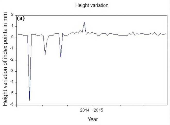
• Figure 6    displays the result of field height variations and histogram inventories with level detector during a year and revealed that the height variations of the study area is non-stationary and some index

points showed downward and upward trend and some data from 100 points omitted because did not show surface dynamic.

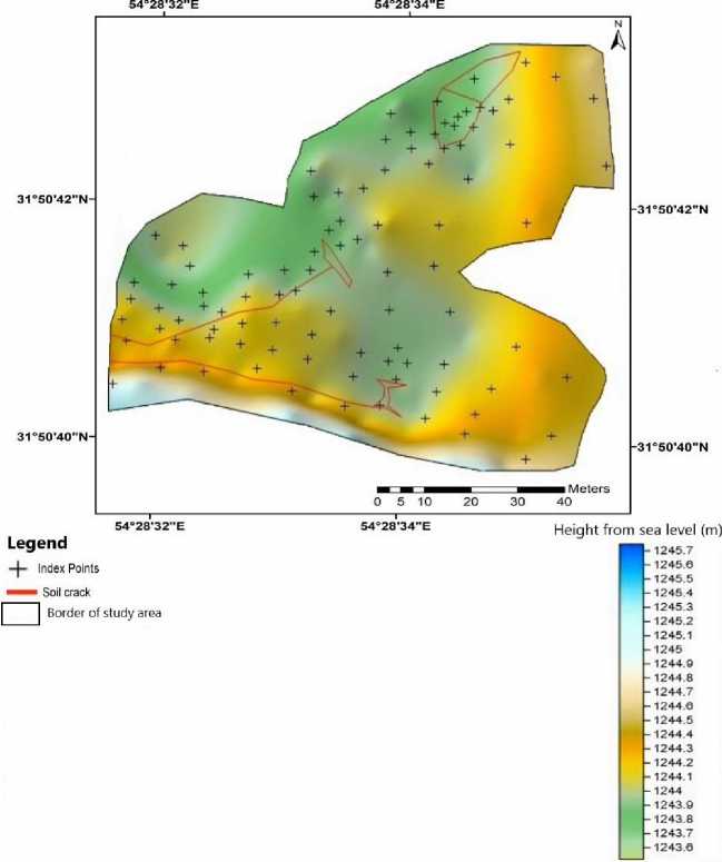
Fig. 4. Topographic map of the study area.

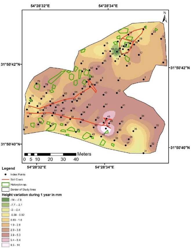
Fig. 5. Height variations of the soil surface in the study area during a year in mm.

Series: Heightvariation difference in ajear

Sample 2014-2015

Observations 77

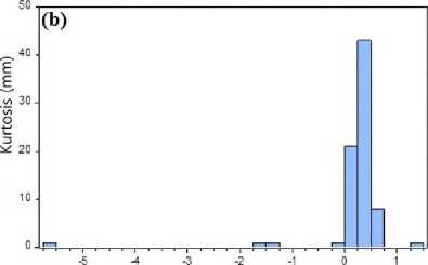
Minimum and Maximum (mm)

Mean        0 206494

Median       0.300000

Ma>imum     1.400000

Minimum    -5.600000

Skewness   -6242551

Kurtosis      46.78243

Jarque-Bera  6650167

Probability    0.000000

Fig. 6. The height variations of the index points during one-year inventory ( a ) and histogram of height variations ( b ).

Selected patterns in this research for time series modeling include 81 patterns of ARMA (AR and MA) model are used to consider maximum degree 8 for AR model as well as degree 8 for MA model (Table 4). By modeling according to the principle of forbearance, the calculation of the Akaike, Schwarz and Hannan-Quinn info criterion were made for the models which presented in Table 4. According to results AR(8) model was the best model.

• Figure 7    shows the results of height variations (Red) and prediction data until year 2020 with AR(8) model and also residual values. According to the diagram below, the AR(8) model fits well on the surveying data.

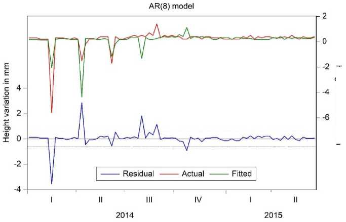
Height variation in mm

Fig. 7. Time series model of AR(8) using surveying data from 2015 to 2020.

Table 5 shows R-squared (R2), Root Mean Squared Error (RMSE), Mean Absolute Error (MAE) and Theil Inequality Coefficient (TIC) parameters of AR(8) model. According to the following results, the model has high accuracy.

Table 4. Akaike, Schwarz and Hannan-Quinn values for modeling height variations data

ARMA order	Akaike	Schwarz	Hannan-Quinn	ARMA order	Akaike	Schwarz	Hannan-Quinn
0,1	2.348	2.44	2.385	4,4	2.435	2.74	2.557
0,2	2.374	2.495	2.422	4,5	2.452	2.786	2.586
0,3	2.4	2.552	2.46	4,6	2.474	2.84	2.621
0,4	2.425	2.6	2.498	4,7	2.5	2.896	2.659
0,5	2.451	2.664	2.536	4,8	2.361	2.787	2.532
0,6	2.475	2.719	2.573	5,0	2.451	2.664	2.536
0,7	2.424	2.698	2.534	5,1	2.477	2.72	2.574
0,8	2.372	2.677	2.494	5,2	2.433	2.707	2.543
1,0	2.348	2.44	2.385	5,3	2.472	2.776	2.594
1,1	2.366	2.488	2.415	5,4	2.444	2.779	2.578
1,2	2.391	2.544	2.452	5,5	2.479	2.845	2.626
1,3	2.416	2.599	2.489	5,6	2.391	2.787	2.549
1,4	2.434	2.647	2.519	5,7	2.475	2.901	2.645
1,5	2.445	2.689	2.543	5,8	2.345	2.801	2.528

Table 4 continued

1,6	2.452	2.726	2.562	6,0	2.477	2.72	2.574
1,7	2.441	2.746	2.563	6,1	2.503	2.777	2.612
1,8	2.324	2.658	2.457	6,2	2.448	2.752	2.569
2,0	2.374	2.495	2.422	6,3	2.497	2.831	2.631
2,1	2.391	2.544	2.452	6,4	2.468	2.833	2.614
2,2	2.414	2.596	2.487	6,5	2.457	2.853	2.615
2,3	2.44	2.653	2.525	6,6	2.478	2.904	2.649
2,4	2.46	2.704	2.558	6,7	2.362	2.818	2.544
2,5	2.432	2.706	2.541	6,8	2.335	2.822	2.53
2,6	2.483	2.787	2.605	7,0	2.5	2.774	2.61
2,7	2.314	2.649	2.448	7,1	2.434	2.739	2.556
2,8	2.351	2.716	2.497	7,2	2.528	2.863	2.662
3,0	2.399	2.552	2.460	7,3	2.47	2.835	2.616
3,1	2.417	2.599	2.49	7,4	2.401	2.797	2.559
3,2	2.381	2.594	2.466	7,5	2.384	2.81	2.554

Table 4 continued

3,3	2.41	2.653	2.507	7,6	2.33	2.787	2.513
3,4	2.43	2.704	2.539	7,7	2.547	3.034	2.742
3,5	2.456	2.76	2.577	7,8	2.27	2.787	2.477
3,6	2.474	2.809	2.608	8,0*	2.193	2.498	2.315
3,7	2.409	2.774	2.555	8,1	2.214	2.549	2.348
3,8	2.361	2.756	2.519	8,2	2.234	2.6	2.38
4.0	2.425	2.608	2.498	8,3	2.26	2.656	2.418
4,1	2.451	2.664	2.536	8,4	2.266	2.692	2.436
4,2	2.462	2.705	2.559	8,5	2.289	2.746	2.472
4,3	2.436	2.71	2.546	8,6	2.296	2.783	2.491
8,7	2.257	2.775	2.468
8,8	2.341	2.889	2.56

Note. * Indicates the best model.

Table 5. The model accuracy of AR(8)

R2	RMSE	MAE	TIC
0.65	0.15	0.11	0.24

• Figure 8    illustrates evaluation between surveying data with AR(8) model and drone data in 2020. The drone after 5 years was able to accurately identify 35 points and adapted to surveying data. Forecasting results of the surveying data until year 2020 have relationship with drone data according to correlation coefficient (R² = 0.6549) between them.

Height variation of AR(8) model and Drone 2015-2020

>

ъ

I

-5

-10

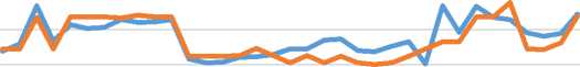
1  3  5  7  9  11 13 15 17 19 21 23 25 27 29 31 33 35

Index points

^^^^^мAR(8) model ^^^^^м Drone

Fig. 8. Comparison between AR(8) prediction model and drone real time imagery in year 2020.

• Figure 9    shows the difference between last inventory height data from surveying (2015) and topography from drone stereo imagery (2020). The height variations of study area varied -150 mm to +78 mm after five years. Also, the height variations near crack lands showed variability after five years. These results displayed that the accuracy of the prediction model is acceptable. This model could be used for areas

  that are similar by the characteristics to the study area.

  
  
  

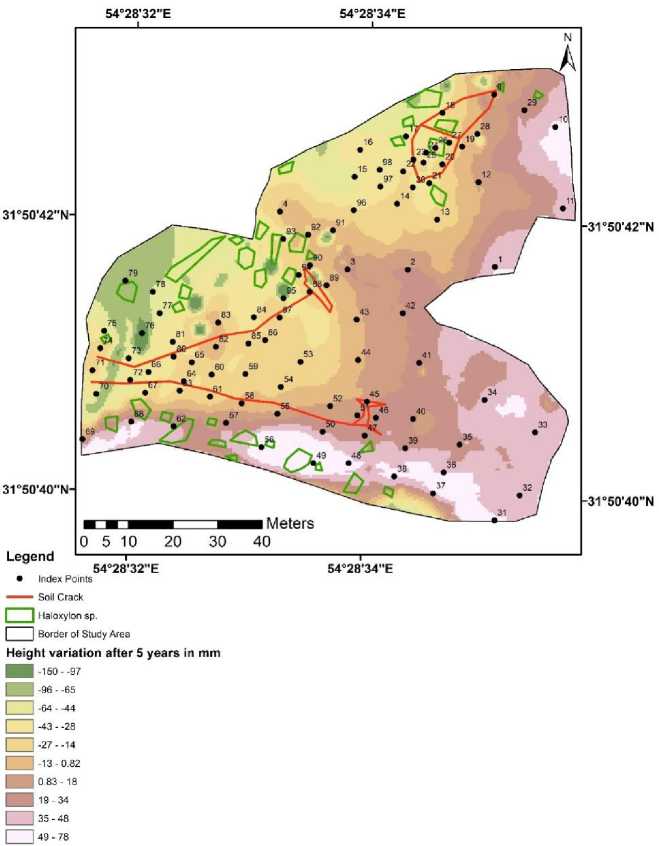
  Fig. 9. Height variations after 5 years (2015–2020) using surveying data (2015) and drone elevation (2020).

  
  

  The height variations in a year obtained from surveying data showed that the region follows indentation and extrusion state and the region is active to extension of soil surface subsidence. Some major factors that is related to soil surface subsidence dynamic movement beside groundwater extraction, including 1) weathering in soil surface leaded to increase in smaller particles content (%clay + %silt) as soil properties (Ekeleme, Agunwamba, 2018; Yang et al., 2019); 2) amorphous materials with more soil dispersion particles (Azarakhsh et al., 2022); 3) the arid climate; 4) suborder soils as calcids and torrerts in the Aridisols and Vertisols orders (Golden, 2014).

In the study area land depressing was related to clay silicate degradation that can accrued with increasing soil alkalinity in the surface horizon up to 9.0. The increase of amorphous silica from 1% in deeper to 7% in the surface horizons of the soil profile (Table 2) confirmed amorphization of clay minerals. This phenomenon of silicates amor-phization occurred in the study area, and monthly changes of soil surface wetting and drying is the core parameter for soil surface subsidence dynamics in contrast to the very deep groundwater level as it is shown in this paper and confirmed by Amin et al. (2019). The soil processes after wetting and drying intervals were led to form microrelieves on the land surface and to appearance of not irreversible deep cracks. Higher alkalinity and salinity in topsoils in comparison to subsoils (Table 2) have been intensified minerals degradation and formation of amorphous materials (Amin et al., 2019).

The height variations in the study area revealed by surveying method fluctuated from -14 to +14 mm/yr1 and by using time series modeling (ARMA) with surveying data, the ARMA model could predict height variations of soil surface subsidence 5 years further. The ARMA model and drone altitude data showed close results for height variations of soil surface subsidence, which were from -150 to +78 mm 5 years further. For validating the prediction accuracy, the ARMA model results were compared to drone altitude data (Figure 8) with the same projected system and finally the ARMA model result was adaptable for forecasting height variations. Also, the drone’s altitude data was suitable for investigating the height variations of observation points with high resolution. These results showed that the study area is active in terms of soil surface subsidence dynamics in vertical direction. Re- searchers worked on time-series of soil surface subsidence rate as downward movement of soil surface subsidence using satellite images in regional scale (e. g. 1 : 150 000 and 1 : 200 000) such as Chen et al. (2015), Su et al. (2021), Ty et al. (2021), their results showed that the study area was active in terms of soil surface subsidence over time because of groundwater extraction and the average rate of soil surface subsidence during 7, 18 and 50 years was 41.43, 42.8 and 31.13 mm/yr, respectively. In this research with intensive study on soil surface subsidence by measuring height variations over time in local scale (1 : 1 000) using surveying method there was found the rate of soil surface subsidence during a year in the study area and in addition to downward movement, upward movement was also observed. The factors of height variations of soil surface subsidence did not change too much during 5 years obviously and the amount of downward movement of soil surface (soil subsidence) was more pronounced than upward movement.

This phenomenon can be related to the higher amount of underground water extraction in the study area, the results of this research is coincide with results of Ilia et al. (2018) and Orhan (2021), they found that the increase in soil surface subsidence was related to significant downward trend in groundwater wells levels and in deformation of the aquifer system due to groundwater level fluctuations. Rahmati et al. (2019), Zamanirad et al. (2020), Mohebbi Tafreshi et al. (2020) investigated the potential zones susceptible to soil surface subsidence, using artificial intelligence model, and their results showed that the major reasons for soil surface subsidence in the studied areas were decreasing ground water level and soil type effects, which is consistent with the results of the present study.

CONCLUSIONS

According to results of this research it can be concluded that two methods of surveying and drone image are suitable for investigating the height variations of the soil surface subsidence and soil cracking, and also time series modeling, such as ARMA model, showed acceptable results. The land in this area had movement in vertical dimensions. As a conclusion to be proposed mapping of the hazardous zones after mineralogy and geochemical analyses as a complementary analysis with mechanical ones to prevent damages in sensitive constructions. According to geochemical and crystal-chemical processes in the soil, the study area is at high-risk of soil surface subsidence because of the clay’s combination with amorphous silicones. The surface cracks with vertical dynamics in the study area are affected by short periods of rainfall and drought, which leads to microrelieves formation on the land surface. It was concluded that to study height variations resulted from soil surface subsidence and soil cracks over time, the best and most appropriate method is combination of height variations data obtained both through surveying and by drone stereo image in a union prediction time series model. It is suggested that this research could be generalized to other regions with similar landforms and soils, which are dependent on ground water, such as agriculture, urban and industrial lands.