Solid Launcher Dynamical Analysis and Autopilot Design

Published Online February 2011 in MECS

The launcher addressed in this study is structured in four stages, three of which are powered by solid propellant rocket motors, whilst the fourth stage is liquid propelled. The first three stages allow bringing the payload and the upper module to the perigee of an elliptic orbit whose apogee is at the final orbiting altitude. The liquid propulsion Attitude and Vernier Upper Module (AVUM) assures, among others, the orbit circularization at the apogee altitude. Vehicle attitude control is achieved by using the grid fins and the direct lateral forces provided by a bipropellant liquid propulsion system allocated in the AVUM module. The physical configuration of the launcher is presented in Fig. 1.

The research of modeling and computer simulation in the filed of space technology has been explored since 1960s and the relative theory and techniques were founded [1]. Dynamic modeling for the object being studied has become the basic step in system design and analysis [2-4]. The mathematic models including centred motion model, roll motion model, switch function model, guide function model and mass function model, etc. were studied by many researchers [5-7]. Besides, some institutes in China, with some conducted predevelopment and experiment on specific models, had explored the modeling and simulation technology in the field of aerospace during 1991-1995 [8].However, these existing models can’t meet the need of the launcher presented above exactly.

grid fins

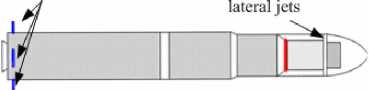
Figure 1. The model of the small solid launch vehicle.

This paper builds on the work presented in Ref. [9-12]. In this paper a complete set of six-degrees-of-freedom dynamic models of the launcher, incorporation its rigid body, aerodynamics, gravity, sloshing, mass change, actuator, and elastic body, is developed on the basis of the Newtonian formulation as it offers physical insight into the interaction between vehicle and the environment. The full dynamic equations are then subjected to flexible modes and bifurcation analysis and the results of these analyses are supplemented using flexible modes sketch maps and bifurcation curves. The presented dynamic models and analysis results can further be used in flight control system design for the small solid launcher.

• II.    R IGID L AUNCHER M ODEL

The six-degrees-of-freedom equations of motion of a rigid body launcher consist of the translational and rotational equations. In an inertial earth reference system, the translation equation of motion of the launcher is md% / dt + m

where m is the mass of actual launcher;

F is the resultant of all the external forces;

v^vis the velocity of the launcher;

Ov is the angular velocity of the launcher.

The considered external forces acting on the launcher are: aerodynamic, gravitational and thrust forces. The forces generated by the attitude engines are omitted while considering the translational motion of the launcher.

In the wind axes frame the aerodynamic force components are

[Fa FyA FzA ]T =[-D L s]T ,                                (2)

where

D is the drag force;

L is the lift force;

S is the side force.

These forces are determined by means of both wind tunnel experimental test and numerical simulations.

The thrust components are easily determinable in the body frame

[FxT FyT FzT]T =[F 0 0]T ,                                 (3)

where FT is the total thrust of the first stage main engine. The profile of the thrust can be obtained from test results.

In the local geocentric frame, the gravitational attraction force is

Fg = m[0 0 |J||]^T ,                                               (4)

where g^vis the gravitational acceleration, which depends on the earth mass gravitational constant, on the distance of launch vehicle from the earth centre, and on the launcher local geocentrical latitude.

The rotational motion of the launcher is equivalent to yawing, pitching and rolling motions about the centre of gravity. In the body frame, the rotational equation of motion is the following v vvv dh / dt + ox h = L ,                                      (5)

where

L is the total resultant of the external torques;

h is the angular momentum of the launcher.

The angular momentum h , expressed in the body frame, is given by

v h = Iov ,                                                      (6)

where

LxT = ^2T0 lxarmkx

LyT   ^T1 lyarmky   ,

LzT = T1 lzarmkz where the lxarm, the lyarm and the lzarm are the distance between the active attitude engine and the current position of the centre of gravity of the whole launch vehicle, and T0 and T1 refer to the forces provided by the attitude engines. The coefficients kx, ky, kz describe the interaction between the main flow and the attitude jet, and they are decided by test results.

• III.    FLEXIBLE BODY MODES

• A. Figures and Tables

P The flexible characteristics of a launch vehicle can be expressed using a beam model representing the lateral and longitudinal motions, respectively. Fig. 2 shows notations used for the analyses. Since the treatment of both motions is similar, only longitudinal motions are adopted in subsequent sections.

Figure 2. Notations for analysis of lateral and longitudinal dynamics.

The moment M(x, t) on the cross section of a beam at position x is represented by

M (x, t ) = EI — x                   f        d2z(f t)A     (9)

= f(f-x)q(f,t)df + f(^-x) -m(f)     2, xx where z(x, t) is the displacement of the cross section at x in the z-direction, EI(x) the bending stiffness, q(x, t) the distributed force in the z-direction, and m(x) the mass of the cross section per unit length. The equation of motion for the lateral dynamics of the beam is

[ Ix 0 0 ~ I = 0 Iy 0 (7) . 0 0 Iz _ d2 [    d2z )     , Ad2z

—7 EI —7 + m(x ) —7 = q(x , t ) .                     (10)

d x ² 1    d x 4     ⁽ ) d t ^{2      (} )                                  ’

The homogeneous equation is defined as is the inertia matrix in the case of a central inertia axes body frame.

The external moments are the aerodynamic and the attitude engine thrust torques. The external moments due to the attitude engine thrust vectoring are d2 [   d2 Z )    2

—7 El - to m x)Z = 0, dx ² (    dx ² J ⁽ )

where the set of eigenvalues and the eigenfunctions satisfy the orthogonal relations

L

J 0 Z_tm ( x ) Z j dx = M i S j

,L    2² (    d ² Z )

Jo Zd T EI-TT dx = M^ S j ( i = U,K)

^J 0 dx \ dx J

.

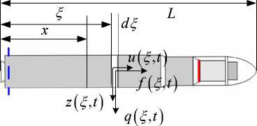
Considering that the distributed aerodynamic force is proportional to the angle of attack and that the z-component of the thrust is proportional to the lateral jet thrust, q ( x , t ) is

q(x,t) = qSCza (x)a + ja(13)

A flexible-body model of launch vehicle is expressed as

I J0      M, JM, where ηi is the ith bending mode.

According to the Newtonian formulation, the free body equation of motions of the slosh masses can be written as:

F. mig cos (9 + ф) = m^px, сф

—ф--mg sin ( e ^{+ ф} ) = m . a pz

l

The equations of motion for the vehicle can be written as follows:

с » ф?

2           2

Fc - mvg sin 9 + E Fsh.s'n ф +E "T2" cos ф = mlvaobzb

=1                    =1

• 2                  2    C ^j*.

  ^- £ bF sM ^{sln Ф -} £ ^b i -^JTc- ^{cos Ф +} F c L c ⁺ £ ^M pi = I Y b ^*

=1                       =1 l=

Thus, Eqs. (15)-(19) form a closed set of equations that govern the dynamics of the coupled slosh-vehicle system.

• IV.    F UEL S LOSHING M ODEL

Sloshing effect is not serious during the solid rocket boost flying phases; as a result, we derive the dynamic model of the upper stage with sloshing effects. Fig. 3 shows a schematic representation of the launcher with two slosh tanks.

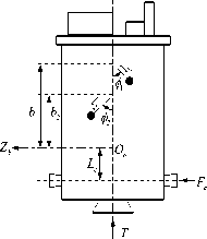
Figure 3. Schematic representation of launch vehicle with slosh tanks.

The X b - Z b system is a set of body-fixed non-inertial axis. θ gives the attitude of the body axis system with respect to the Earth fixed frame. The slosh tanks are modeled by equivalent pendulums of length l i hinged at a distance b i from the centre of gravity of the non-sloshing mass of the system. Ф i is the angles of rotation of the pendulums with respect to the body x -axis. The acceleration of the vehicle centre of gravity is given by the following expressions:

a_o x = * + ^V_z , ^ao z = V - ^x                     (15)

Ob Xb     x z Ob Zb     z x

V. A NALYSIS R ESULTS

The above sections have discussed dynamic models that the launcher is expected to be encountered. Such as rigid body, aerodynamics, gravity, sloshing, mass change, actuator, and elastic body models. In this section, we will give some dynamic analysis results based on these models.

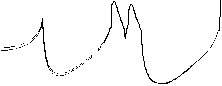
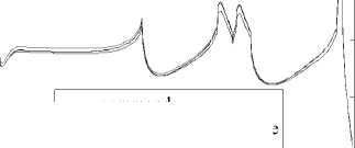
Since the launcher possesses the characteristics of a long and slender body, its flexibility should be considered carefully. Usually, modal frequencies, displacement, and rotation are given from an engineering software (such as Nastran) solution and is used to model the interaction effects between vehicle flexibility and the other dynamic models. As discussed in section 3, lateral vibration is the dominate vibration mode. It is important to consider the effect of this vibration in control system design due to the modal frequencies being near the control bandwidth. The vehicle’s elastic motion can be conveniently expressed in terms of frequencies and mode shapes of a free-free beam structure. Because of the axial symmetry of the launcher, two identical modes exist in the lateral bending. Fig. 4 gives the dominate vehicle mode shapes.

The expressions for accelerations of the pendulum masses are given as follows:

a px = l. ^ T ) 2 + ao_bx_b cos Ф . — a o_bz_b sin ф - b^&^ cos Ф . + b, & in ф . a pz. = 1 . 1^*' & ) + а о ь Х ь sin Ф + a O b Z b cos Ф . - b , * 2 sin ф . - b . & cos ф

The slosh damping moment of a single pendulum is given by the following relation:

M_pi = С ф ф

(a) First bending mode.

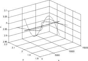
(b) Second bending mode.

Figure 4. Visualization of the first three structural modes shapes.

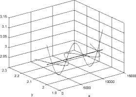
(c) Third bending mode.

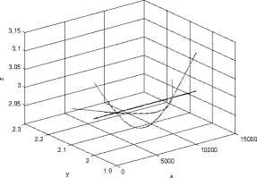
Slosh-vehicle coupling can lead to instability in the launcher in planar flight. The coupled system has been modeled using a multi-body formulation in Section IV. We shall be presenting the results of bifurcation analysis for the launcher. Fig. 5 shows the locus of Hopf points in ε 1 - ε 2 space.

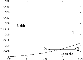
Figure 5. Hopf point locus.

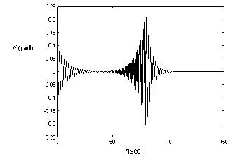
Figure 6. Time History of Slosh Amplitude.

The neutral stability curve divides the space into two parts. A system with two tanks can show interesting behavior depending on the order in which fuel in the tanks is used. Consider, for example, the path 1-2-3 shown in Figure 5. This path shows a typical drain-out plan with one of the tanks being drained after the other tank. The points 1 and 3 are both stable. However, while going from configuration 1 to 3 the system intermediately passes through unstable configurations. Thus, a stable-unstable-stable type of behavior in a simulation corresponding to this drain-out plan is expected. The result of such simulation is shown in Fig. 6.

• VI.    A UTOPILOT D ESIGN

• A.    Constrained Optimization Filter Design

P It has been previously demonstrated in multiple space applications that bending filters can be designed numerically using a constrained optimization framework. The design parameters are the coefficients of the bending filters. Consider the following attitude and rate filter

П ^{S + 2} x 4 i + 2 x 4 i + 1 ^{S +} x 4 i + 1

F att ( ^S 7 = 11 2,o             , 2

t = 0 ^{S  + 2} x 4 , .+4 x 4 i + 3 ^{S +} x 4 , ₄3

^S + 2 x 4 i + 2 x 4 i + 1 S + x 4 i + 1

F rate ( ^S /11 2,o              ,2

i = 0 ^{S + 2} x 4 i + 4 x 4 i + 3 ^{S +} x 4 i + 3

A set of feasible parameters must satisfy the following constrains:

C1-The filter itself must be stable and minimal phase to guarantee stability and performance.

C2-The bandwidth of the bending filter should be greater than that of the PID controller to avoid rigid performance degradation.

These constrains can be used to set the upper and lower bounds for the bending filter design.

The primary objective of the control system design is to provide sufficient stability margins in the presence of various parameter uncertainties while maintaining adequate system response. The stability margin criteria include:

O1-The closed-loop control system must be robustly stable under mass property, slosh, and atmosphere variation.

O2-Gain/Phase margin requirements for the nominal system, the perturbed system and the bending modes should be satisfied.

O3-Control systems must also ultimately demonstrate robustness to uncertainties in the plant.

The goal is to design bending filters that are robust to uncertainty in structural frequency, mode shape, mass properties, and aerodynamics characteristics.

Once design objectives and constrains are identified, the bending filter design task is ready to be cast as the following constrained optimization problem min x E R4 n, G

^{f (} x )

s . t .

g ( x ) <0

x l <  x <  x u

The filter design criteria C1 and C2 can be formulated as inequality constraints. These inequality constraints can be also cast as objectives in the above multi-objective constrained optimization problem. In general, these objectives are competing to each other. There is no unique solution to this problem. Pareto optimality must be applied to characterize the objectives. This is accomplished with a weighted sum strategy, which converts the multi-objective problem into a single objective optimization problem.

• B.    Autopilot Design Based on State Dependent Riccati Equation

State feedback controllers, such as the PID controller, the Lyapunov-function-based quaternion feedback controller and the LQR state feedback controller are commonly used in the missile autopilot design. The LQR method is well developed for linear systems with optimal performance and good stability. However, the motions of missile systems are highly nonlinear. [16-19] The linearization near the equilibriums of interest will introduce system errors; sometimes deteriorate the system performance and stability. SDRE nonlinear regulation is one of the options of using an extension of LQR theory on nonlinear problems [13]. It is a nonlinear control system design methodology for direct synthesis of nonlinear feedback controllers. By turning the equations of motion into a linear-like structure, this approach permits the designer to employ linear optimal control methods.

State Dependent Riccati Equation method developed by Cloutier et al. [13,14] is to construct nonlinear feedback control laws for nonlinear systems. The main idea is to represent the nonlinear system x = f (x) + B (x) u(22)

in the state-dependent coefficient (SDC) form x = A (x) x + B (x) u(23)

and to use the feedback u = -R-1 (x) BT (x) P (x) x,(24)

where P(x) is obtained from the SDRE

P ( x ) A ( x ) + A T ( x ) P ( x ) -

P ( x ) B ( x ) R ¹ ( x ) B T ( x ) P ( x ) = - Q ( x )

and Q(x) and R(x) are design parameters that satisfy the condition Q(x)≥0, R(x)>0 for all x. As the equation of motion has been turned into a linear-like structure, LQR method can be employed to make it an optimal regulation problem. Define the quadratic performance index in state dependent form

J = 0.5/ 0 ° ^ x^TQ ( x ) x + u T R ( x ) u ] dt .               (26)

The state dependent weighting matrices Q ( x ) and R ( x ) can be chosen to realize the desired performance objective. Some of the nomenclature associated with the SDC parameterization is given to aid in the presentation of the stability theorem.

The launcher on-board computers require discrete-time models for implementation. The SDC matrices [ A ( x ), B ( x )] are transformed into a discrete-time system using a sampling period of T

G = exp (A (x (k)) T)

H = (jTexp(A(x(k))r)dr)B(x(k)).(28)

The SDRE becomes

P ( x ( k )) H ( x ( k )) + H^T ( x ( k )) P ( x ( k )) -

P (x (k)) G (x (k)) R-1 (x (k)) GT (x (k)) P (x (k))

= ^- Q ^{( x ( k} ))

and the feedback will be

u ( k ) = - R ^{- 1} ( x ( k ))( x ( k )) H T ( x ( k )) P ( x ( k )) x ( k ) (30)

Thus, every step can be numerically implemented.

The SDRE method requires full-state feedback, but in practical situations, measurement of all the system states might be neither possible nor feasible. Launcher-borne sensors have to measure all these states to realize the SDRE controller. But, in practice, the some of them are sometimes not measured in order to simplify the on-board sensors and reduce cost. Such situations would demand the need for some observers or dynamic compensators which would make the overall system more complex. Since the output is available, output feedback can be realized using fast output sampling (FOS) [15]. FOS feedback has the feature of static output feedback and makes it possible to arbitrarily assign the system poles. Meanwhile, FOS feedback always guarantees the stability of the closed-loop system. Thus, the SDRE-based controller can be implemented while not all the state variables can be measured.

Fast Output Sampling (FOS) is a static output feedback methodology to realize a given state feedback by using a multi-rate observation of the system output signals. In FOS, each sampling period T is subdivided into N subintervals

A = T / N .                                 (31)

N must be chosen greater than or equal to the observability index of the system and a constant control signal is applied over a period T .

Consider a plant described by discrete-time linear model of the form x (k +1) = Gx (k) + Hu (k)

control problem, choose the appropriate system states ⁽³²⁾          and form the SDC factorization.

y ( k ) = Cx ( k )

where x e Rⁿ , u e R m , y e R p and G , H and C are of appropriate dimensions. Here ( G , H ) and ( G , C ) are assumed to be controllable and observable respectively. Let ( g , h , C ) denotes the system ( G , H , C ) sampled at rate 1/ A viz.

x ( kT + ( j + 1 ) A ) = gx ( kT + j A ) + hu ( kT ) , j = 0, 1, , L , N -1

and the output measurements are taken at time instant t = kT + jA, j = 0, 1, ,L, N-1. According to [3], yk+1 = Cо x (kT) + Dо u (kT)                      (35)

where yk+1 = [У(kT) У(kT + A) L У((k + 1)T -A)]T

C 0 =[ C Cg L Cg^{N - 1} ] T

D о = 0 Ch C ( gh + h ) L

N -2   . "1 ^T

C Z g-h

and x (kT ) = Lyyk + Luu ((k -1) T)                      (37)

where

L y = G ( C T C о ) ^{- 1} C T

L u = H - L y D о

.

Thus, the last N output samples and a constant control signal can be used to estimate the system states of the slower sampled system.

To implement the SDRE method on the launcher motion model presented in the former section all the system states in the dynamic equation are required by the controller. The FOS method is used to estimate the states needed in order that only the output of the system, which is available, is used to generate the control action and that the system state matrix is renewed in every control interval.

The procedure of the design of the SDRE based autopilot using the FOS method can be summarized into the following steps. It takes the assumption that the initial system states used in the SDC is known.

Step 1 . Choose the SDRE control step T and the numbers of subintervals N so that every control period T is subdivided into N subintervals, calculate A using (31). Meanwhile, choose a fictitious measurement matrix C .

Step 3 . Choose the proper Q ( x ) and R ( x ) to calculate the control signal u by means of the SDRE method.

Step 4 . Transformed the SDC obtained in step 2 into discrete-time systems using the sampling periods of T and A . Thus, we get the system matrix G , H and g , h needed in (32) and (33).

Step 5 . Measure the output samples y_k for each of the T intervals and using the same control signal calculated in step 3 in current interval. Use the FOS technology express in section 2 to estimate the next system states of the slower sampled system.

Step 6 . Go to step 2 to calculate a new SDC for the system.

Thus, a calculate circle has been made and for each longer sample time T a control signal is obtained.

The effect of the above algorithm is illustrated with an example.

The initial state is x0 =[0. 1 0.01 2.5 -0.01]T .(39)

The weighting matrices for the simulation are chosen as constants.

Q = diag ([100 100 23 100])

and

R = 6 x103.(41)

Perform all the steps numerically on Matlab will get the simulation results.

The simulation results are illustrated as Fig. 7 - Fig. 9. Fig. 7 shows the response of th e angle of attack and Fig 8 shows changes in fin defection with respect to the simulation time. These results are satisfactory. The designed controller is very effective in tracking the commanded trajectory. The system is stabilized by the controller. Fig. 9 compares the states and control response under the condition that the system parameters have 150% uncertainties and 50% uncertainties. The results show that the designed controller has good robustness.

Step 2 . According to the dynamics of the satellite attitude

command response

4    6    8    10   12   14

Time (sec)

Figure 7. Attitude angles without noise.

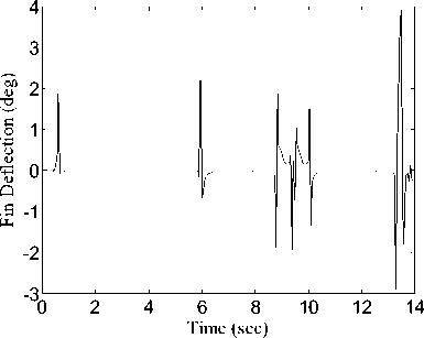
Figure 8. Attitude angle rates without noise.

Oil

о

Oil я

-2

command system parameters have 150% uncertainties system parameters have 50% uncertainties

-4 I ¹                                       I I                                       ¹                               1

0     2     4     6     8    10    12    14

Time (sec)

Figure 9. Control torques applied to the satellite.

• VII.    C ONCLUSIONS

A set of dynamic models of a small solid launcher, incorporating its propulsion, aerodynamics, sloshing effects, and structural flexibility, has been described in this paper. The preliminary results of flexible modes and sloshing bifurcation analysis have been discussed. The study purpose was to develop a complete set of dynamic models for the performance and stability analysis of the launcher. These models are based upon the Newton’s law and can further be used in flight control system design, simulation and analysis.