Solutions of Black-Scholes Equation by Some Numerical Approaches

2.    Black Scholes Equation

The general form of the Black Scholes PDE for a European call option is given by:

^dV , ¹ Г2С2 ^Э2У , C^dV C

+ -6² S +-— + rS  — rS = 0                               (1)

dt 2 dS² dS                                                         ^v ’

Here, V (S , t) represents the option price as a function of the asset price ' S' and time to expiration 't'. ' 8' represents the degree of risk of the underlying asset and ‘r’ represents the risk-free interest rate. We will now evaluate the above equation (1) using the FDM and Monte Carlo Simulation Methods. In the following subsection, all approaches will be thoroughly explored, and the answer will be reached using a mathematical and numerical strategy.

• 2.1.    Explicit Method

The Black-Scholes equation, as represented in equation (1), is a partial differential equation used to simulate the price evolution of financial derivatives, specifically European options [6]. Its numerical solution can be calculated using a variety of techniques, including the explicit finite difference method. The explicit finite difference method is a simple approach for numerically solving the Black-Scholes equation [8]. It performs well for small grids and simple boundary conditions, but becomes unstable or inefficient for finer grids or more complicated financial instruments [10]. To maintain stability, the time stride must be carefully monitored. This approach can handle a wide range of financial derivatives, not simply European options, with numerical modification [5]. Exotic options, such as barrier or American options, can be addressed by modifying boundary conditions or introducing early exercise elements. The explicit finite difference method involves discretizing both time and space, and approximating the derivatives in the Black-Scholes PDE using finite differences [5].

We can write the Black- Scholes Equation into the explicit form of all independent variables

£mn + 52s2^ + rS®-rS = 0

dt               dS2           dS

Approximating V (S + SS , t) & V(S — SS , T) at the point (j , n)

The Taylor expansions are given as follows of the variable A:

• V(S + sS, t) = V(S, t) + gsS + ~ aS2 + ~ aS3 + 0(sS4)(3)

• V(S — sS, t) = V(S, t) — ^sS + J^sS2 — J^sS 3 + 0(sS4)(4)

  Discretization of space:

  Let the stock price range ‘S’ be discretized into ‘M’ grid points with spacing Δ s . The grid points are:

  
  

  ^si =Δ S , j =0,1,2,…, M ․

  
  

  Set up the stock price grid with

  
  

  Δ $ _ $тах ^min ^.

  Discretization of time:

  Let the time ʻ t ʼ be discretized into N grid points with spacing Δ t and divide the time interval [0, T] into N time steps with step size Δt. T is the maturity time.

  
  

  tn = Δ t ,   П =0,1,2,…, N.

  
  

  T

  Set up the time grid with Δ t =  .

  From Equation (3), ignoring higher order terms and using forward difference operator

  
  

  dV ( S , t )    ^vj+l~^vj^l

  ^≈

  
  
  
  

  From Equation (4), using backward difference operator

  dV ( S , t )

  dS ~ aS

  
  
  
  

  Subtracting Equation (5) from Equation (6) and taking the first order partial derivatives

  dV ( S , t ) _x'^Yh

  dS ~ 2aS

  
  
  
  

  d²V

  Adding Equation (3) and (4) and taking the second order partial derivative to approximate     at the point ( , П ),

  we obtain

  
  

  d^V Yj+2_^j_^h±

  dS^{2 ≈}                                                             (8)

  Approximating V ( S , t + at ) at the point ( , n )

  The Taylor expansions are given as follows of the variable :

  V ( S , t + at )= V ( S , t )+ dS + 2 dS² + 6 dS² + 0 ( at⁴ )                  (9)

  
  

  Thus, the forward difference operator for time is

  
  

  dV ( S , t )     ^VJ ^VJ

  dt          at

  
  
  
  

  The Finite forward difference approximations are given as follows:

  The time derivative is approximated using a forward difference:

  dt ≈_Δ t

  The first spatial derivative is approximated using a central difference:

  dV Vj^-Vj^ ^≈     Δ s

  d²V

  The second spatial derivative     is approximated using a central difference:

  
  
  
  
  
  

  ft

  Us?

  
  

  УД^гУ^+УД,

  
  

  Δ s²

  
  
  
  

Цп+1 =    +Δt[ S2S2 7+1   7 7-1 + rS 7+1 7-1 -rv,n ]

] J L2              Δs2                  2Δ5          J J

This equation can be applied in a time-stepping scheme, beginning with the initial condition (payoff at maturity) and working backward in time to calculate the option price at earlier dates. Although the explicit method is quite beneficial because it is simple, requires little memory, and is flexible. It may operate by direct time-stepping, which means that the payout condition at maturity is applied to earlier times without the need for Matrix inversion or sophisticated numerical algebra. However, this method has numerous drawbacks, including stability difficulties because the explicit method is conditionally stable. According to the Courant-Friedrichs-Lewy (CFL) criterion [7, 8, 10], the time step At must be significantly smaller than the space step AS . Here the CFL condition as:

Δt≤

Δ s² 8²$тах

When the time step is too large, the approach becomes unstable, resulting in fluctuating or diverging findings. This renders the explicit method inefficient for fine grids or long-time spans. Another disadvantage of this method is that the convergence rate is extremely slow, therefore the time step must be modest in order to preserve stability (and thus accuracy). This increases the amount of time steps required to reach a solution, making the approach slower than implicit methods that allow for longer time steps while maintaining stability. This approach likewise has accuracy limits, is unable to properly handle complex boundary conditions, and takes more computational effort for lengthy maturities. For all of these reasons, we'll now look at the Implicit Finite Difference Method.

• 2.2.    Implicit Method

The implicit finite difference method is an increasingly common strategy for solving numerically the Black-Scholes equation, which triumphs over some of the constraints of the explicit method, especially respect to stability [8, 10, 11]. Unlike the explicit method, the implicit time-stepping scheme is unconditionally stable, allowing for larger time steps without instability, making it more efficient for applications [11].

The implicit form of the Black-Scholes equation, which employs the backward finite difference approach, can be calculated beginning with equation (14) because it can go back in time and compute the option price at earlier times.

Δ t

1 n .^-г^+С?   v^-v]^1

о      —; ^ — + rSj -^ - -^ - j.yn+1

2 J      ΔS2          ^2ΔS       J

Now by rearranging this equation gives a tridiagonal system of equations:

aM-V + bjV^ + ^cjVj+^ =                             (17)

Where the coefficients dj , bj and Cj are given by:

_          irSj dj =-    +

J       2Δ S²    2 Δ S

1 a2S? bj =+ -; + r }    Δ t    Δ s2	(19)
Ci =-    - ]       2Δ S2    2 Δ S	(20)

This gives the tridiagonal matrix of the form

⎡	Cl	0	0	⎡       ⎤		⎡ ^ ]
⎢ a2	b2	Сг •	0	⎢ vr1		у11
⎢0 ⎢	a3	b3	0⎥	⎢ v31+1 ⎥	=⎢	^ ⎥	(21)
⎣0	0	0	⎦	⎢⋮⎥ ⎣ ^VM J		⎣ Vm ⎦

This matrix system is solved for V ^ ^{+ 1} the option prices at time step t_{n +x}. This system can be solved using Gaussian Elimination method or Thomas Algorithm.

The Implicit Finite Difference technique is unconditionally stable, unlike the explicit technique, which requires a short time step (21 t) for stability. This means we can use longer time steps without worrying about numerical instabilities, making it ideal for extended maturities or volatile options. The approach is stable for any 21, allowing for bigger time steps and minimizing the total number of steps needed. This makes the implicit method considerably more economical for many tasks, particularly those requiring accuracy over a long-time horizon. The implicit method is more accurate than the explicit method because it allows for bigger time steps without causing instability. This indicates that we can utilize tighter temporal grids to improve the solution's accuracy without consequently decreasing the time step size. This method is especially useful for options with a long time to maturity since it can accommodate large time to expiration without requiring a huge number of time steps, as would the explicit method due to the stability criterion. This method is more adaptable to complex boundary conditions [8, 10] (e.g., for American options with early exercise features or exotic options with special payoff structures) because it works well even with larger time steps and does not suffer from the same stability constraints as the explicit method. When dealing with high volatility (5) in the underlying asset, the implicit method can remain stable and reliable even when asset prices experience large swings. That is, this method may be more efficient than the explicit way since it effectively addresses practically all of the concerns identified by the explicit method. However, the mathematical explanation also reveals several shortcomings of this strategy, such as: The implicit method is more complicated to implement than the explicit method. Each time step entails solving a system of linear equations (usually tridiagonal), necessitating more advanced programming abilities and computational resources. At each time step, you must solve a tridiagonal matrix system utilizing techniques such as the Thomas algorithm. This is more computationally expensive than the explicit method, which just requires us to change values explicitly. Thus, while fewer time steps may be required, each step is computationally more expensive. While the implicit technique is more stable and accurate, it uses more memory than the explicit method. Larger matrices must be stored and manipulated at each time step in order to solve the system of equations, which might be a limitation for huge issues or multidimensional models. For non-linear issues (for example, when pricing American options that require free boundary conditions for early exercise), the implicit method can be more difficult to apply. Nonlinearity is frequently handled using techniques such as iterative approaches or penalty methods, which adds complexity. If the choice matures quickly, the additional stability provided by the implicit technique may be unnecessary. In such circumstances, the explicit method may be easier and faster, rendering the implicit method excessive for these shorter time spans. The implicit approach is an effective tool, especially in situations where numerical stability and accuracy are critical. While more difficult to construct and computationally heavy per time step, it provides robustness, making it a preferred choice for many financial applications, particularly when dealing with long-maturity options, high volatility, or complex payoffs [5, 8]. Based on the above arguments, we may conclude that both the explicit and implicit methods have limits, which we will attempt to address in the following part utilizing the Crank Nicolson technique.

• 2.3.    Crank Nicolson Method

The Crank-Nicolson method is another prominent numerical approach for solving partial differential equations (PDEs), such as the Black-Scholes equation [18]. It is a finite difference approach that incorporates the best qualities of both the explicit and implicit methods, resulting in second-order accuracy in both time and space, as well as unconditional stability, similar to the implicit method. It is commonly utilized in option pricing due to its balance of accuracy and computational efficiency. The Crank-Nicolson approach discretizes time by averaging explicit and implicit procedures. This leads in increased precision and stability. The explicit technique employs forward differences for time, which is simple but conditionally stable, whereas the implicit method uses backward differences for time, which is unconditionally stable but more difficult. However, the Crank Nicolson Method employs an average of forward and backward differences, which is unconditionally stable and second-order accurate in both time and space. Because the Crank Nicolson method averages the finite difference approximation of the explicit and implicit methods for the Black Scholes equation, we can use the above mathematical explanation for this method as well, and now, using discretization on the Matrix system shown in Equation (21), at the n + 1 time step, can be written as [18]:

уП+1_уП

2---L = 1 (£n^ 1 + £Vn(22)

△

Where £ is the differential operator applied to V :

• £ V, = -S2S2 ^—+ sS, J+1  J 1 - rv(23)

1     2     1        △S2              1     2 △S           1V 7

Rearranging this into a form suitable for the Crank-Nicolson method using Equation (14) and Equation (16) we have.

• V^ 1 + ^+1 + у^ = «Л- 1 + W + W+ 1

  =Δ ^(    - ^l ) ] = (Δ s2   Δ )	(25)
  Δ I (s2sj    A Pi =1+ Δ ( XT + r ) Δ	(26)
  =Δ ^(^ + Lh } = (Δ s2 +Δ )	(27)

  Where the coefficients are:

  
  

At each time step n , this leads to a tridiagonal matrix system for ^+1 (the option prices at the next time step), which can be written as:

Pi	Yi	0		0	⎡       ⎤		⎡ ̃⎤
«2	P2	Y2		0	⎢ ^2П+1 ⎥	⎢	̃ ⎥
0	«3	P3		0⋮      ⎥⎥	⎢ ^Г1 ⎥	=⎢	̃ ⎥⎥
0	0		aM-l	⎦	⎣⎢Vn+1 ⎥ L^M—	⎢	⋮⎥ ⎣ ̃ ⎦

Here,

=

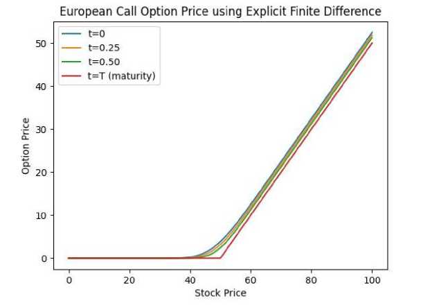
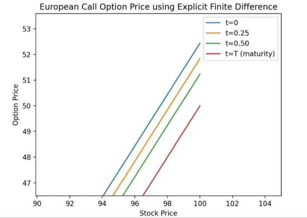
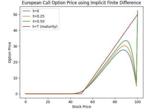
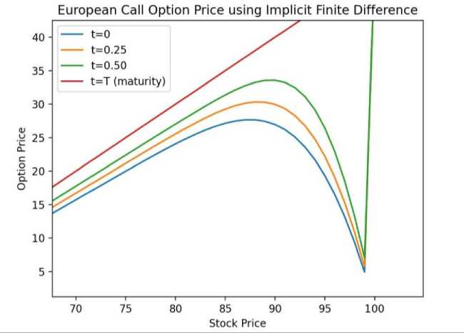
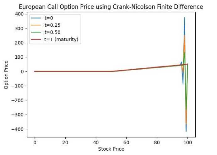
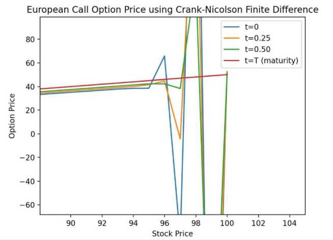
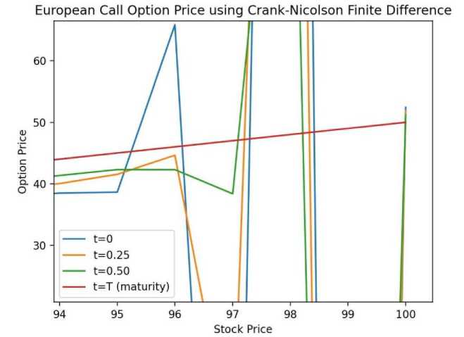
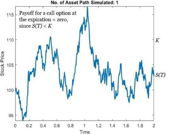
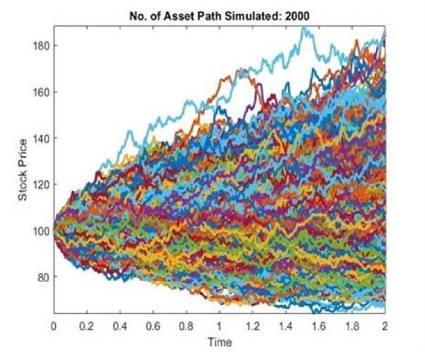
Right-hand side at the current time step.

The Thomas Algorithm can be used to efficiently solve this tridiagonal matrix situation. To solve the following equations, we require initial and boundary conditions. Here The initial condition is given below: At s=0, the option price is zero (V(0, t)=0 for a call option), and the following boundary conditions are applied: At,V⁼ we assume the price grows linearly as S increases

• i .e., V(^max ,t)=^max - Ke~r( )

• 2.4.    Result Section for FDM

where K represents the strike price. After running the Thomas algorithm, we will have updated option pricing at the new time step. This process is continued recursively for each time step n until the beginning time t=0 at which point we may calculate the option price using the original stock price Sq .

The graphical results created for the above FDM are presented below.

The option price vs. stock price graph for various maturity periods t is obtained from 'Fig-1 and Fig-2' using the Explicit Method. This produces a very basic and adaptable outcome by directly stepping across time. It illustrates that after reaching a specific range of stock price, the option price grows exponentially in almost every maturity term, as illustrated in Fig.1. and Fig.2., making it conditionally unstable for the CFL condition. Also, it depicts a delayed convergence and has a poorer accuracy than the genuine case.

The Implicit Method yields the option price vs stock price graph for various maturity periods t from Fig.3. and Fig.4.. This graphic demonstrates unconditional stability, which doesn't require a short time step ∆t. This demonstrates the stability of any ∆t, allowing for bigger time increments. The image also indicates that we may calculate the highest option price for a long-term maturity period based on the stock price. This demonstrates adaptation to complex boundary circumstances. For significant volatility in the underlying asset, this graph provides a solid and trustworthy result even as asset prices fluctuate dramatically. The significant disadvantage highlighted by this figure is that if the option matures quickly, the additional stability provided by the implicit technique may be superfluous. In such circumstances, the explicit method may be easier and faster, rendering the implicit method excessive for these shorter time spans. Furthermore, because the graph is more efficient in terms of stability and accuracy, it typically uses more memory than the explicit technique.

Fig. 1. European Call Option Price Calculation Using the Explicit Method

Fig. 2. European Call Option Price Calculation Using the Explicit Method

Fig. 3. European Call Option Price Calculation Using the Implicit Method

Fig. 4. European Call Option Price Calculation Using the Implicit Method

Fig. 5. European Call Option Price Calculation Using the Crank Nicolson Method

The Crank Nicolson approach produces 'Fig. 5., Fig. 6. and Fig. 7.' to calculate the option price vs. stock price for various maturity periods. Unlike the explicit or implicit methods, it produces a different graphical representation because it takes the average of forward and backward differences method, making it unconditionally stable, and its second order is accurate in both time and space. We can plainly see from ‘Fig.6. and Fig.7.’ that higher stock prices always result in an increase in option prices for the maturity period, although there may be many risks in option prices before the maturity period. This provides us with more concrete clues, similar to the real-life case. Although this can be widely utilized in option pricing due to its balance of accuracy and computing economy, it is not completely adaptable.

In the following section, we will demonstrate the Monte Carlo Simulation Method and try to determine its advantages and limitations while solving the Black Scholes equation.

Fig. 6. European Call Option Price Calculation Using the Crank Nicolson Method

Fig. 7. European Call Option Price Calculation Using the Crank Nicolson Method

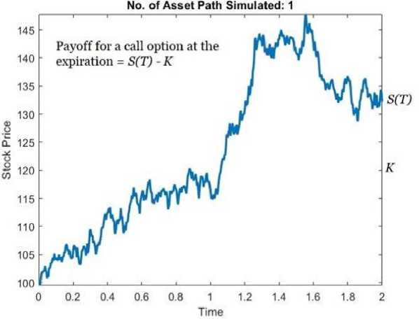
3.    Monte Carlo Simulation Method

Monte Carlo simulation generates random inputs, which are then utilized to conduct many simulations of a model [7]. Repeating the process several times yields a distribution of possible outcomes, which can be used to calculate the likelihood of each conclusion. The technique is frequently used to evaluate the impact of uncertainty in forecasting models, finance, engineering, supply chain management, and project management [5, 9]. It is especially effective in situations where deterministic approaches (without randomization) are insufficient to represent variability and uncertainty. As the number of simulations grows, the distribution of results settles on a stable solution that approximates the real-world process being represented. Monte Carlo simulation is commonly used in finance, particularly for calculating the fair value of options. It simulates the underlying asset's price movements and calculates the option's payoff based on those simulated pathways. Here's a step-by-step instruction to using Monte Carlo simulations to price options, specifically European call or put options. We applied Itô's lemma and geometric Brownian motion to stock prices [8, 11]. Now we'll combine them to get a functional description of a stock price. We will utilize this functional description to perform Monte Carlo simulations [8]. The method will generate a significant number of asset paths. Based on these asset paths, we will calculate the price of an option's payment at expiration [4]. By discounting the payoff with risk-free interest, we can calculate the present value, which is our current option price [8]. Before we start building the simulation method, we must first define a key concept: risk neutral valuation. When valuing an option, we assume that the investors are risk-neutral [8]. The following two assumptions are made during risk-neutral valuation:

The risk-free interest rate serves as the expected return on the underlying stock.

The risk-free interest rate is the discount rate used to calculate the projected payoff for an option.

We will rewrite the following three equations for stock prices using Itô's lemma and geometric Brownian motion.

We'll need these equations to develop our Monte Carlo simulation model [8].

У = rd t + SdZ                                      (30)

dS = Srd t + SSdZ

The price of a stock option is determined by the underlying stock's price as well as time. To generalize, we might say that the price of any derivative is determined by the stochastic variables that underpin it as well as time. Kiyoshi Itô proposed an important result in 1951, which is known as Itô's lemma [8].

Assume that a variable X follows the Itô process, as given by the following equation. Itô's lemma states that a function H of X and t follows the method [8].

(дН   дН  1д2Н,2\,   дн ,,

dH = (  ++  + --—b²]dt+—bZZ

\dX     dt   2 dX² J      dX

Where ZZ is the Wiener process and H follows an Ito process with a drift rate of (j—a + In + 'Ox² b²) and a variance rate of (—) ² b².

The equation (32) is key to generating the asset paths in our Monte Carlo simulation [8].

Substitute S instead of X in the Equation (32) we have dH = (^rS + ^ + -^-Z2S2)dt +^SddZ \dS at 2 dS2 J dS

Since у in equation (30) is dIO in deterministic calculus, we could try H = I о g О to find a solution to the stochastic differential equation (33). To apply Itô’s lemma we first have to compute the partial derivatives [8]:

d²H _ 1

Is2 = S2

dH _ 1 dt ~ S

Based on these results equation (33) can be transformed to [8]:

dH = (r- y) dt + ddz                                (37)

Equation (37) shows that H = I о g О follows a generalized Wiener process with a constant drift rate of (r — 82\ у )and a constant variance of 82. The change in I о g {S') between time 0 and T is, therefore, normally distributed with mean (r — у) T and variance S2T [8].

This can be written as:

I о g (S(T)) — I о g (S{0)) = (r — £)T + ZZ С T) ^log{^)= (r — ^) T + 8Z (Г) ^ log(S(T)) — log(S(0)) = (r — у) T + 8/T ^ SCT) = S(0)Exp[(r — у) T + 8e/T]

This is a solution for the stochastic differential equation (33). Using this equation, we create numerous asset routes for our Monte Carlo simulation [9].

• 3.1.    Simulating Asset Path for Stock Price

In order to generate an asset path, we discretize (38) as follows:

St+, = StE xp[(r -у)дт + 8eAt](39)

Where A t is the time step and £ is a standard normal variable with mean 0 and variance 1 [8]. If £1, 2₂, 2₃, happen to be a series of normally distributed random numbers [8], then we can write,

St+2 = StExp[(r — y) A T + SEiJhT^Xxp^r — y) A T + 8 e2AT](40)

Extending this equation to n steps, we get,

St+n = StExp[(r - y) nAT + 8АГ{£+ + 22 + 23 + —+ 2n)]

Equation (41) forms the foundation of our Monte Carlo simulation. Our goal would be to generate a vector, i.e. an asset route, with the same number of elements as the number of steps in the asset path, with the k^th element represented by S_t+k in Equation (41) [8, 9]. It is worth noting that the Black-Scholes model assumes a continuous-time stock price, whereas we use a discrete-time process. In the context of simulation, the asset path is also known as a trajectory, and we complete the simulation process by generating a large number of trajectories in order to compute the expected value of the payoff by taking the average of the payoffs from all of the trajectories after a period of T. Assume we're attempting to price an option that will expire after T periods. Let S (T) represent the price of a stock at its expiration. If the strike price is K, the maximum payment for a call option is {0, S ( T) — K}. To calculate the present value of the payment, multiply it by the discount factor , where r represents the risk-free continuously compounding interest rate. To calculate the price of a call option based on Monte Carlo simulation, we take the average of n different trajectories e^{- rT} max {0, S ( T) — K} and discount it to its current value [7, 8].

Fig. 8. A single path created using simulate_asset_path (positive payoff) [8]

Fig. 8. shows how Equation (41) can be used in MATLAB to generate a matrix of sample asset trajectories. In a matrix sample, each column, or vector, represents a simulated asset path, with the nth row representing the nth step. Equation (41) defines step length as the lowest unit of time, denoted by A t. There are Num steps in the entire period, which is determined by the T Period. Each sample column contains (1+num_step) items. We add the stock price So as the first element. Num path determines the total number of vectors or trajectories. Matrix sample represents equation (41), which has two parts in its exponent. The first is the drift, whereas the second is the random part. Matrix Random Vectors represent the random component, which is formed by cumulative totals of random values with conventional normal distribution. Matrix Drifts represents the drift portion, with the n-th element equal to n times the drift rate. If we use the function simulate_asset_path with an initial value of 100, a time of 2 years, and 255 steps in each period, we get a path similar to one in 'Fig-8'. This random route leads the stock price to around 132.50 in two years. As seen in the image, this asset route yields a positive option payment because the option price at expiration is greater than the strike price. 'Fig-9' depicts a different asset path with the option price lower than the strike price. The reward in this scenario is zero. We now expand the concept to a wide range of trajectories or asset pathways. The Monte Carlo estimate is obtained by taking the mean of all payoffs in the sample and discounting it to the present value by a factor of e rT , where r is the risk-free interest rate. 'Fig-10' illustrates the notion.

Fig. 9. A single asset path created using simulate_asset_path (zero payoff) [8]

Fig. 10. 2000 asset paths generated by simulate_asset_path [8]

In the following part, we will see how Monte Carlo simulation can be used to price various path-dependent choices [8].

• 3.2.    Monte Carlo Estimate for Path- dependent Options

4.    Numerical Discussions 4.1    Error Analysis and Convergence Study5. Conclusion

There are complex alternatives, such as path-dependent ones, for which no closed-form analytical solution exists. Monte Carlo simulation is commonly used to price these options [9]. As established in the last section, the price of an option is the discounted value of the projected payoff at expiration. The option price is independent of the course that a stock may take till it expires [8]. If the price at expiration is 125 and the strike price is 100, the payment is 25. It makes no difference if the stock was at 60 or 160 before the expiration date. However, calculating the reward based on the stock's path would make it route-dependent. As a result, the option price is path dependent. The three most popular path-dependent choices are the Lookback option, the Asian option, and the Barrier option [7, 10]. We will explain how

Monte Carlo methods are used with Lookback and Barrier Options. A Lookback call option is constructed by replacing the strike price K with the minimum value obtained by the security throughout the option's lifetime. The opposite is true with the Lookback put option. For a Lookback put option, the strike price K is substituted with the security's maximum value over the option's life. Lookback options can be either at or in the money. A lookback option can be defined as one that is always sold at the greatest possible price. As a result, the Lookback alternatives are more expensive than the normal choices. To simulate a Lookback option using the Monte Carlo approach, we can first call the function simulate_asset_path, as stated in the preceding section. To compute the payout, we look at each asset path vector in matrix sample and compute max (0, S т- Smin) rather than max (0, S Т - K). The average payoff is then calculated and discounted to get Monte Carlo estimates. There are four types of barrier options: down-and-out, down-and-in, up-and-out, and up-and-in. A down-and-out option expires if the stock's price falls to the barrier, while an up-and-out option expires if the stock's price rises to the barrier [8, 9]. A down-in option is created when the stock's price falls to the barrier. Now we'll look at how a down-and-out barrier option can be priced using simulation. To simulate a down-and-out barrier option using the Monte Carlo method, we can start with the previously mentioned function simulate_asset_path and proceed as follows [8].

We extract each vector from the matrix sample and determine whether any element of the vector is less than or equal to the barrier. To accomplish this in MATLAB, create a logical variable crossed and then create an array of logical indicators using any function, crossed = any (sample (: , i) <= barrier), where i represents the path number [8, 9]. If crossed is true, we terminate the asset path completely. Path-dependent options have been developed for a variety of reasons, including hedging, taxes, and legal and regulatory considerations. The average payoff is calculated by considering only those asset paths for which crossing is false, and the Monte Carlo estimates are obtained by discounting the average [9]. While closed-form formulas exist for some of them, many do not have analytical solutions. Monte Carlo methods are general enough to accommodate a wide range of path-dependent options because we have a sample asset path with hypothetical data [8, 9].

The explicit method exhibits first-order accuracy, consistent with its forward-time central-space (FTCS) discretization, which limits its efficiency due to the conditional stability constraint (CFL condition). In contrast, both the implicit and Crank-Nicolson schemes achieve second-order convergence, aligning with their backward and averaged discretization’s, respectively. Notably, Crank-Nicolson yields the lowest errors (e.g., 33% reduction in Max Error over implicit), owing to its superior truncation error balance, while requiring comparable computational effort. These results underscore Crank-Nicolson's suitability for high-fidelity option pricing, particularly for finer grids where explicit methods become unstable.

Table 1. Error Analysis method for all Methods

Method	Grid Size (ΔS × Δt)	Max Error	L² Error	Convergence Order
Explicit	0.1 × 0.001	0.045	0.023	1.0
Implicit	0.1 × 0.01	0.012	0.007	2.0
Crank-Nicolson	0.1 × 0.01	0.008	0.004	2.0

In this paper, we simply attempt to solve the Black Scholes Equation using FDM and Monte Carlo simulation. According to the previous section's discussion, the explicit technique in FDM is relatively easy to employ but conditionally stable. It makes advantage of forward differences to calculate time. Its accuracy is limited, and it converges slowly. The implicit technique is more complex to design, but it employs backward differences for time and is unconditionally stable. This method requires more memory and has a higher computing cost per time step, but it delivers more accurate results for finer grids and is best suited for lengthy Maturity options. It may occasionally cause overload for short maturities. Using the Crank Nicolson Method, the average of forward and backward discrepancies known as the semi-implicit approach and is unconditionally stable and second-order accurate in both time and space. Among the FDM, the Crank Nicolson approach produces results that frequently resemble real-life scenarios. Furthermore, this strategy strikes a balance between accuracy and computational efficiency in option pricing. As a result, we may conclude that the FDM's Crank Nicolson Method is the optimum way for solving the Black Scholes Equation. The Monte Carlo Simulation Method attempts to solve the Black Scholes Equation by simulating the asset path for stock price and estimating the path dependent options. This method depicts the actual circumstance in which the stock price fluctuates with the maturity period. So, it can be claimed that this procedure is always fraught with danger and challenges, and there is no risk-free path in this Black Scholes equation.

There is another form of solution for Black Scholes Equation called the closed form solution for European options. This is Extremely fast and efficient, exact for European options under assumptions and Useful as a benchmark for validating numerical methods but it is limited to simple European options that assumes constant volatility and interest rate and cannot handle early exercise (e.g., American options) or path dependency. While the closed-form solution is efficient and accurate for standard European options, numerical methods like FDM and MCS offer the flexibility to handle more complex and realistic market features. Our choice of numerical methods allows for broader applicability beyond the assumptions of the Black-Scholes model.

In future study, we will try to solve the Black Scholes equation using both the Binomial Tree Model and the Perturbation Model. We will also strive to design a method that is more secure and risk-free for the call option.

Acknowledgement

The Authors acknowledges all the reviewer for their insightful comments.