Solving of the inverse diffraction problem in the first Rytov approximation for retrieving the phase object dielectric permittivity

The inverse diffraction problems play a crucial role in studying various phase objects exposed to coherent laser radiation and more. Phase objects can arise in the form of plasma formations with an extremely rapid evolution in time and space [1, 2], shock waves [3, 4], turbulent flows of gas or liquid [5], complex condensed media [6], biological cells and tissues [7], optical fibers [8], etc. Generally, the object under study can appear as an optically inhomogeneous and non-isotropic medium, in which in addition radiation absorption can occur. Hereinafter, we exclude other complex nonlinear effects caused by the interaction of probing radiation with the probed object [9,   10]. To reconstruct optical characteristics (refractive index or dielectric permittivity) of a three-dimensional phase object, methods of phase diffraction tomography are used [11, 12]. When using a single angle of probing, the object characteristics are often retrieved assuming the axial symmetry of the object and further considering, e.g., the classical inverse diffraction problem in the geometrical optics approximation [13]. This problem is closely related to the numerical solution of the inverted Abel integral equation [17, 18, 19, 20, 21]. When reconstructing the object characteristics, it is important to consider diffraction effects as accurately as possible. To this end, modeling of the Maxwell’s equations [14] is employed or the scalar Helmholtz wave equation [13] is solved with using the expansion of the wave field into analytical basis functions [15, 16] or other various asymptotic approximations, e.g.,

18287/2412-6179-CO-1617.

the first Rytov and Born approximations. One of these approximations, which has proven itself in practice, is the so-called first Rytov approximation. This approximation together with the first Born approximation forms a single family of the key asymptotic approximations [22]. Multiple studies [23, 24, 25, 26] show that the first Rytov approximation provides reliable data when modeling the direct problem of diffraction of laser radiation by complex-structured phase objects. This approximation also allows one to evaluate diffraction effects accompanying the passage of probing radiation through a phase object and behind its output plane [27], the description of which significantly goes beyond the limits of classical approaches [2]. When neglecting diffraction effects, a significant distortion of the reconstructed object characteristics whether in a modeling or full-scale experiment can be obtained. In this regard it is of interest to construct such a solution of the inverse diffraction problem, which is not computationally demanding, while being sensitive to the accompanying diffraction effects.

In this study, we concern one of such solutions for an axisymmetric phase object both with and without radiation absorption based on the results of solving the scalar Helmholtz wave equation in the first Rytov approximation. In this approximation we derive computationally efficient equations, which take into account diffraction effects accompanying the wave passage through the object and enhancing in free space. The fundamental properties of the obtained equations are discussed together with their broad applications.

1.    Basic equations for evaluating wave diffraction

Let us consider the diffraction problem for a model phase object in Fig. 1(a) exposed to a plane optical wave. The object is characterized by dielectric permittivity s(x, p) = 1 + s(x, p) (here p is the two dimensional variable introduced for variables y and z), wherein the second term serves as a dispersive part (depends on the radiation wavelength) and can be complex (when radiation absorption occurs in the object). In the study we assume the object to have axial symmetry in the YZ plane with the coordinate of x = R (R denotes the object radius) and be probed by plane wave I0 exp(ikx) propagating along the Ox axis. Hereinafter, we omit factor exp (- iю t). The wave has parameters: intensity I0, modulus of wave vector k = 2п / X, and wavelength к The wave passage through the object is accompanied by diffraction, and wave intensity I(x, p) and phase shift 8ф(x, p) undergo changes. The object is surrounded by an infinite medium with a uniform dielectric permittivity equal to unity. In this medium behind the object the diffracted wave continues to propagate.

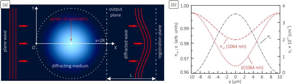
Fig. 1. (a) Schematic representation of the wave diffraction problem for a phase object with axial symmetry. (b) Properties (n e electron density, s dielectric permittivity, and n ref refractive index) of a model plasma filament 20 g m in diameter exposed to a plane wave at 1064 nm

We describe wave diffraction by the phase object by considering the scalar Helmholtz wave equation with the employment of the first Rytov approximation [28]. Assuming all the key criteria for the applicability of this approximation to be satisfied, we arrive at the following equation

%(x,fp) = -k^(x', fp)e^x-x)f2dx'.(1)

2 i ⁰

Here functions T 1 ( x , f _p ) and Л ( x ', f _p ) are defined as

Л( x, ft,) = j'Js ( x, p) e "2 ” ipfp d 2p,

%(x, f>) = Jf®. (x, p) e-2 ”ipfp d2 p,(3)

where function Ф 1 ( x ,p) appears as the Rytov’s complex phase

Ф1 (x, p) = ikx + i 8ф1 (x, p) + %. (x, p).(4)

In the presented equations function 8ф 1 ( x , p ) describes the acquired phase shift of the diffracted wave, and function X 1 ( x ,p) = ln ( yj1 1 ( x , p ) / 1 0 ) is understood as the wave level and characterizes the changes in the wave intensity. The variables f_y and f_z are the spatial frequencies connected with the coordinates y and z , and f _p appears as the two-dimensional variable introduced for f_y and f_z . From Eq. (1) the phase shift and intensity of the diffracted wave are found as 8ф 1 = Im ( T ^{- 1} ( ^ 1 ) ) and 1 1 = 1 0 x exp ^ 2 x Re ( T ^{- 1} ( ^ 1 ) ) ] , where symbol T ^{- 1} stands for the inverse Fourier transform.

Finally, we note that, although Eqs. (2) and (3) imply the use of the Fourier transform in transverse planes, functions Л ( x , f _p ) and T 1 ( x , f _p ) themselves do not present the direct Fourier transforms. In essence, e.g., function Л ( x , f _p ) appears as a set of the Fourier spectra obtained for each section of function s ( x , p ) having the longitudinal coordinate of x .

2.    Solution of the inverse problem for a real dielectric permittivity

Let us consider first the phase object without radiation absorption. In the case at hand, function s ( x , p ) is real, and Eq. (1) can be represented as ^ ( x , f , ) = T ( x , f , ) + iH ( x , f p ), where

H ( x , f p p ) = -2 £ x cos ( Xn ( x - x ') f 2 ) Л ( x ', f ,) dx ', (5) k ^x

T ( x , f p ) = - £ sin ( Xn ( x - x ) f p ² ) Л ( x , f p ) dx . ⁽⁶⁾

Functions H = T(5ф1) and T = T(x1) denote the two-dimensional Fourier spectra of the wave phase shift and level distributions, which are defined behind the object in a certain YZ plane with the coordinate of x = 2R + L (serves as a parameter). Here L denotes the distance from the object output plane to the plane, in which the level and phase shift spectra of the diffracted wave are defined. Let us move the origin of the coordinate system in Fig. 1(a) to the object center and introduce new parameter x = R + L and integration variable x" = x'- R . By performing simple transformations of trigonometric functions in integrals (5) and (6), the latter can be represented in the following form н (x, fp) =

= k cos( Xn xf 2 ) j cos( Xn x 'f 2 ) Л ( x ‘‘ , f _p ) dx ‘‘ , T ( x , f p ) =

= k sin( Xn xf 2 ) j cos( Xn x "f 2 ) Л ( x ‘‘ , f , ) dx ‘‘ .

Since both equations have the same kernel of the integral transformation,

R

θ(fρ)=    cos(λπx′′fρ2)Λ(x′′,fρ)dx′′, it is sufficient to consider only one of these equations to solve the inverse problem, i.e. reconstruct function ε by using the level and phase shift spectra of the diffracted wave.

Let us turn to function θ ( f _ρ ), which performs a nonstandard cosine transformation of function Λ ( x ′′ , f _ρ ) along the longitudinal coordinate x ′′ , and introduce three-dimensional Fourier transform Λ ( f_x ′′ , f _ρ ) of function ε ( x ′′ , ρ )

Л ( f x ‘‘ , f ,) = JJJJ ( x ‘‘, p ) e ^{- 2 n} i( x ^f "^{+p f} ’⁾ dx ‘‘ d ² p . (9)

One can notice that function θ ( f _ρ ) is related to function Λ ( f x ′′ , f ρ ) as follows

θ ( f ρ )=¹ Λ ( f x ′′ , f ρ )| _{f = f} 2 _{λ /2}= 2                ^{x ρ}

= ^+∞ Λ ( x ′′ , f ρ ) e ^{-π ix ′′ f ρ 2 λ} dx ′′ .

-∞

According to expression (10), function θ ( f ρ ) can be understood as a three-dimensional Fourier transform of ε ( x ′′ , ρ ), which is defined not in the entire frequency space, but on the surface of paraboloid f x ′′ = f ρ ² λ /2. By taking the advantage of this fact, we write Eq. (7) in the following form

2 k -1 H ^{( x} L , ^f, ^)sec ( Xk ^x L ^f2 ) = Л ( f x ,^f p ) | x=f^/2 . ⁽¹¹⁾

Let us assume function s ( x ‘‘, p ) to have spherical symmetry. Then its three-dimensional Fourier spectrum also has spherical symmetry in the frequency space, and the function on the right side of Eq. (11) can be represented as

Λ ( f x ′′ , f ρ )| _{fx ′′ = f ρ} 2 _{λ /2}= Λ ( ( λ f ρ ² /2) ² + f ρ ² ) .

In the case of cylindrical symmetry of the object, whose function ε ( x ′′ , ρ ) does not have a gradient along the Oz axis, we have

Λ ( f x ′′ , f ρ )| _{fx ′′ = f ρ} 2 _{λ /2}= Λ ( ( λ f y ² /2) ² + f y ² ) .

The Fourier spectrum of the phase shift is H ( x l , f _p ) = H ( x l , f y ) 8 ( f z ), where 8 ( f z ) is the delta function, as well. Let us use the idea that any inverse diffraction problem is an ill-posed problem, and, hence, it is inevitable to employ certain approximations to construct an appropriate solution of the problem. In our consideration we simplify function Λ ( f x ′′ , f ρ ) for the cases of two types of symmetry. By transforming Λ ( f_x ′′ , f _ρ ) on the right side of Eq. (11) to the form of Λ ( f ρ λ ² f ρ ² /4 + 1 ) , we estimate the value of λ ² f _ρ ² /4. The reasoning below also applies to the case of cylindrical symmetry, i.e. Λ ( f_y λ ² f_y ² /4 + 1 ) . The maximum value of spatial frequency f _ρ can be estimated from above by using parameter l _ε , which is of the order of s /1 V s | (here we have V = h i ^x d / d x + h i y д / d y + h i z д / d z ) and coincides with object radius R . Following this way, we have λ ² f _ρ ² /4 ≤ ( λ /2 R ) ² . If the key conditions for the applicability of the first Rytov approximation are satisfied, i.e. with l s >  X (see the details in Ref. [27]), quantity ( X /2 R ) ² <  1 turns out to be of the second order of smallness relative to unity, and function Λ ( f x ′′ , f ρ )| _{f ′′ = f} 2 _{λ /2} on the right side of Eq. (11) can be represented ^ρ with a high accuracy as Λ ( f _ρλ ² f _ρ ² /4 + 1 ) ≈Λ ( f _ρ ). Thus, the right-hand side of Eq. (11) is nothing more than the two-dimensional Fourier spectrum of function ε ( x ′′ , ρ )

2 k' H ( x l , f, )sec ( Xn x L f pP ) = Л ( f , ).              (12)

In fact an accuracy, with which the left and right sides of Eq. (12) coincide, depends on the relationship between the geometric aspects of the object and wavelength of probing radiation that can be checked only numerically. It is expected that the equality of the right and left sides in Eq. (12) is fulfilled with an accuracy, with which one can in principle trust the results of modeling wave diffraction in the first Rytov approximation, see the examples in Refs. [12, 26]. Yet, if the equality of the left and right sides in Eq. (12) is observed with an accuracy, which does not entail a significant error in reconstructing function ε ( x ′′ , ρ ), for Eq. (12) it is possible to determine an unique solution to the inverse problem. Let us take into account the fact that in the case of axial symmetry (both spherical and cylindrical) spectrum Λ ( f _ρ ) can be related to ε ( x ′′ , ρ ) through a zeroth-order Hankel-transform operator [29]. So, for the case of cylindrical symmetry we obtain the solution of the inverse diffraction problem in the form of

s ⁽ r ) =

₄ π +∞                                         (13)

= — L H(xl, fy)sec(XnxLfy) J0 (2nrfy)fydfy, k0

+∞

H ( x L , f y ) = 2 j ₀ 5ф ( x l , y )cos ( 2 n yf y ) dy .         (14)

Here r = x ′′ ² + y ² is the modulus of the radius vector drawn from the center of the object symmetry.

In a similar way we obtain the solution of the inverse problem for the case of spherical symmetry s (r ) =

+∞

= k ^{- 1} Jo H ( x L , f ’ )sec ( ^n x L f y ) sinc( rf p ) f 2 ^df p ,

+∞

H ( X L , f, ) = 2 n J 0 J o ( 2 n f , ) 5ф ( X L , Жd ^ .       (16)

Here we introduce the variable ξ = x ′′ ² + y ² and function sinc( rf ρ ) = sin( rf ρ ) / rf ρ . The variable f ρ = f y ² + f z ² is understood as the modulus of the radius vector drawn from the center of the object’s Fourier spectrum pattern.

Notably, the solution of the inverse diffraction problem can be determined in a similar way by using the level spectrum of the diffracted wave for any x L ≠ 0. For illustration we present the corresponding solution for the case of cylindrical symmetry only

S ^{( r} ) =

4 π ^+∞

= — £ T ( X L , fy )cosec ( ^п X L f y ) J 0 (2 n rf y ) f_ydf_y , k ⁰

+∞

T ( X L , fy ) = 2 J 0 X 1 ( X L , y )cos ( 2 п yf y ) dy .           (18)

3.    Solution of the inverse problem for an imaginary dielectric permittivity

If radiation absorption occurs, the object dielectric permittivity and its sets of the two-dimensional spectra can be written in the form of s ( x ‘‘ , p ) = S i ( x ‘‘ , p ) + i s 2 ( x ‘‘ , p ) and Λ ( x ′′ , f _ρ ) = Λ ₁( x ′′ , f _ρ ) + i Λ ₂( x ′′ , f _ρ ). By substituting functions Λ ₁ and Λ ₂ in Eq. (1), we obtain the following equations

0 1 ( f ,) = H ( X L , f, ) cos( Xn X L f 2 ) +

+ T ( X L , f p )sin( Xn x L f 2 ),

0 2 ( f ,) = H ( X L , f, ) sin( Xn x L f 2 ) -

- T ( x l , f, )cos( Xn X L f p ² )

where functions

R

θ j ( f ρ )= k   cos( λπ x ′′ f ρ ² ) Λ j ( x ′′ , f ρ ) dx ′′

(with j = {1, 2} ) are introduced to simplify the notation. By solving Eqs. (19) and (20) together and using approximations

θj(fx′′,fy)|fx′′=λfy2/2≈θj(fy), the inverse diffraction problem for the case of cylindrical symmetry is solved as

+∞

S j ( r ) = 4J 0 j ( f p ) J o (2 п rf y ) f_ydf_y 0

with j = {1, 2},

where functions θ _j ( f _ρ ) are expressed in terms of the wave level and phase shift spectra defined by Eqs. (19) and (20). Functions H ( x L , f _ρ ) and T ( x L , f _ρ ) are specified in accordance with expressions (14) and (18). In the case of spherical symmetry we have θ j ( f x ′′ , f ρ )| _{f ′′ = λ f ρ} 2 _/2 ≈θ j ( f ρ ), and the problem’s solution is found as ^ρ

+∞ sj (r) = 44 0j(fp )sinc(rf p)f,2dfp with j = {1, 2}.

Function H(xL ,fy ) is defined in accordance with y expression (16), and function T(xL ,fy ) has the form of

+∞

T ( x L , f, ) = 24 J 0 (2 n f p ) X 1 ( X L , ^ d ^ .         (23)

Thus, by simultaneously measuring the intensity and phase shift of the diffracted wave in an experiment, one can reconstruct the complex dielectric permittivity of the investigated object.

4.    Fundamental consequences of the obtained equations

The obtained Eqs. (13 – 23) provide a means for reconstructing the object dielectric permittivity by using the experimentally measured intensity and phase shift of the radiation diffracted by the object. If there is no radiation absorption, the object dielectric permittivity can be retrieved using both the phase shift (this is a standard procedure similar to solving the inverted Abel integral equation [17, 18, 19, 20, 21]) and intensity of the transmitted radiation. This makes Eqs. (13 – 18) more practical and allows for a significant simplification of the entire procedure of reconstructing the optical characteristics of a phase object, since, e.g., in an experiment there is no need to organize a complicated system of laser interferometry to record the object phase patterns. The latter play a decisive role in the established methods for solving the inverse diffraction problems.

In experiments the intensity and phase shift of the transmitted radiation are recorded in a particular plane behind the object with the coordinate of xL . In the case of lensless diffraction optics [30, 31] a CCD matrix is placed directly in this plane and records the brightness diffraction pattern of the object. If distance L from the object to the CCD matrix is known alongside with the object scale (its radius R ), one can immediately retrieve the object dielectric permittivity using the brightness diffraction pattern. This approach, however, has certain limitations associated with the restrictions imposed on the applicability of the first Rytov approximation, when describing wave diffraction behind the object output plane over long distances. We discussed in detail these restrictions earlier in Ref. [27]. The corresponding restrictions should be checked with respect to each object under study taking into account its size and the radiation wavelength.

These considerations are also relevant for the case when the phase object is probed by laser radiation using a lens optical system. The latter can be focused on the object itself ( x L = 0 ) or certain plane behind the object ( x L >  R ), and even in front of it ( x L <  - R ), see more in Ref. [27]. The obtained Eqs. (13)–(23) have trigonometric factors, which introduce corrections to the integrals if we have L ≠ 0 . When the lens system is focused on the object center, fairly simple equations are derived to retrieve the object dielectric permittivity (for illustration we present them for the case of cylindrical symmetry only): when there is no radiation absorption

+∞

s(r) = —J H(0,fy)Jo(2nrfy)fydfy,(24)

k ⁰

and when absorption occurs

+∞ si (r ) = П'1H (0, fy) Jo(2n rfy) fydfy,(25)

k ⁰

+∞ s2(r) = -k-1 f T(0, fy)Jo (2nrfy)fydfy.(26)

In the latter situation one can see that it is possible to completely reconstruct the complex dielectric permittivity only if the intensity and phase shift of the diffracted wave are simultaneously recorded in the experiment. The real part of the dielectric permittivity is uniquely determined by the integral transformation applied to the phase shift spectrum, see Eq. (25), whereas its imaginary part is determined by the integral transformation applied to the inverted level spectrum, see Eq. (26). The Eqs. (24 – 26) itself are closely related to the cycle of the Abel-Fourier-Hankel transformations [32].

The Eqs. (24 – 26) can be used only if the phase shift and level spectra are determined in the plane of symmetry of the object passing through its center. By the way, if the phase shift and level spectra were initially recorded in a certain plane behind the object, they can be determined directly in the object center using the spectral convolution, which describes the propagation of the wave angular spectrum in free space [33]. Previously, based on this approach, we were able to create a highly efficient method for localizing the object in space with the employment of the results obtained with a single angle of the object probing [27, 34]. After localizing the phase object in space and determining the level and phase shift spectra of the diffracted wave in the plane passing through the object center, solving of the inverse diffraction problem is greatly simplified.

Note that Eqs. (13 – 23) together with their representations (24 – 26) can serve as powerful tools of fast and computationally simple testing the phase object for the presence of radiation absorption. If we assume the absence of absorption, the equation connecting the level spectrum with reconstructed function ε(x′′, ρ) should yield a distribution identical to that obtained when solving Eq. (13) with xL ≠ 0 . If the reconstructed distributions do not coincide, then one can consider a model with radiation absorption and solve the corresponding equations for ε1 and ε2 .

5.    Numerical simulations and verification

Let us illustrate the efficiency of the obtained equations by simulating the diffraction problems (direct and inverse ones) for a plane wave (at 1064 nm) passing through a model phase object. This we consider to be a plasma cylinder (with a diameter of 2 R = 20 µ m), with its properties (plasma electron density n e , dielectric permittivity ε , and refractive index n ref , see them in Fig. 1(b)) being taken as close as possible to those of thin plasma filaments observed at the point anode after the electrical breakdown of an air gap in [35]. The electron density profile is taken to be n e ( y ) = A (1 + cos( π y / R )) / 2 (here A = 3.5 × 10 ¹⁹ cm^–3 is the dimension factor; the filament has axial symmetry in x = R ) and related to the filament’s dielectric permittivity as ε =1 -ω ² pe / ω ² , where ω pe = (4 π e ² n e / m e ) ^1/2 ( e and m e are the electron charge and mass) and ω are the plasma and radiation frequencies, as well as ε = -ω ² pe / ω ² . The model filament is exposed to the probing wave (no absorption is assumed to occur), which experiences diffraction and is registered (e.g., by a lens optical system) in a certain plane somewhere behind the filament output plane.

Fig. 2 demonstrates the results of modeling the direct diffraction problem described by Eq. (1). More exactly, in Figs. 2(a) and 2(b) there are the simulated maps of the intensity and phase shift of the diffracted wave obtained starting from the object’s input plane ( x = 0), see also the behavior of the intensity and phase shift profiles plotted along the Ox axis in Figs. 2 c and d . Importantly, when calculating Eq. (1) and performing the Fourier transform of the functions used, the resultant scale of the computational grid should be controlled so that no intersection of spectral tails occurs. For example, the maps in Fig. 2 were obtained on a scale of 2000×400 µ m with a grid step of 1 µ m both in the transverse and longitudinal directions. With these modeling parameters, the convergence of integral (1) was achieved as well. It is seen that wave diffraction results in the emergence of numerous fluctuations in the wave intensity and phase shift. The general pattern of the intensity map is that a significant drop in the wave intensity (plasma filament acts like a negative cylindrical lens) is observed along the wave path behind the filament, whereas in the periphery the pattern is characterized by alternating zones with an increase or decrease in the wave intensity falling within a diffraction cone, the apex angle of which coincides with the area containing the filament. The phase shift pattern is also characterized by numerous fluctuations, and its maximum value is reached in the filament’s output plane. As the distance from the filament increases, the object’s brightness and phase patterns become more distorted.

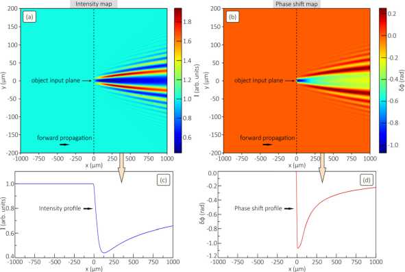
Fig. 2. Panels (a) and (b) demonstrate the intensity and phase shift maps of the wave passing through the plasma filament considered in Fig. 1(b). Panels (c) and (d) illustrate the behavior of the intensity and phase shift profiles along the Ox axis. The plane with the coordinate of x = 0 corresponds the object input plane; λ = 1064 nm

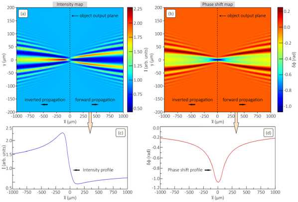
Fig. 3. Panels (a) and (b) demonstrate the intensity and phase shift maps of the diffracted wave obtained by solving Eqs. (7 – 8). Panels (c) and (d) illustrate the behavior of the intensity and phase shift profiles along the Ox axis. The plane with the coordinate of x = 0 corresponds the object center of symmetry; X = 1064 nm

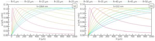
Fig. 4. Panels (a) and (b) demonstrate the behavior of the a = Xn x l f y variable for the cases of two wavelengths (X) and different object radii (R)

The maps in Figs. 3a and b together with the intensity and phase shift profiles in Figs. 3c and d are obtained by simulating Eqs. (7) and (8) and characterize the diffracted wave behavior. Here a number of the fundamental features can be distinguished. The right side of each map equals to that shown in Figs. 2a and b. Directly in the filament center the object is invisible in terms of the intensity changes, whereas its phase shift reaches the maximum value and is uniquely related through the integral transformation to function s(x, p). Remarkably, relative to the filament center the left and right sides of the phase shift map coincide. Opposite to this, the intensity inversion occurs on the left side of the filament center, i.e. the primarily zone with the intensity enchantment becomes the zone with the intensity attenuation. This is clearly illustrated by the curves in

Figs. 3 c and d . In [27] we showed that the discussed features of the wave behavior can be also obtained in terms of the Hopkins and Goodman theory of the object image formation in a lens system. The later can be focused on a certain plane behind the object output plane, directly on the object center, or even in front of it.

Finally, note that the computational capacity of Eqs. (7) and (8) is significantly less than that of the original equation (1), while the predicted results are, in general, the same (outside the object) and more informative (owing to the presence of a region inside and in front of the object).

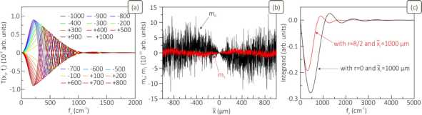
Fig. 5. (a) Spectra T ( x L , f_y ) of wave levels χ ₁( x L , f_y ) obtained with the frequency step of 25 cm^–1 for different x L taken in [–

1000 µ m, …, + 1000 µ m]. (b) The zero-order m ₀ and first-order m 1 moments of level function χ ₁( x L , f_y ) calculated at x L = 0 . (c)

Integrand T ( x l , f_y )cosec ( Xn x i f ) J ₀ (2 n rf_y ) f_y

in Eq. (17) computed with r = 0 and x l =1000 цm or r = R /2 and x l =1000 цm;

λ = 1064 nm

Let us now discuss the computation features of solving the inverse diffraction problem. With respect to the considered plasma filament the solution of the inverse problem is determined by Eqs. (13), (14) alongside with Eqs. (17), (18). On the first glance, the integrands in Eqs. (13) and (17) have singularities, when the variable a = Xn x l f y2 takes the values of ±n /2 , ± 3 n / 2, ± 2 n , ± 5 π /2, etc. However, its absolute value is much less than n /2 with any x l and f_y . Let us show this, with the wave diffraction spreading taken into account. The latter affects the maximum value of the spatial frequency with meaningful information far from the object output plane. Near this plane the frequencies containing the useful information of the object can be limited from above by f^max ≤ 1/ R . At the distance from the object output plane of L the frequencies can be limited from above by f^max ≤ ( R +λ / R × L ) ^{- 1} , where factor λ / R characterizes the diffraction spreading. With X ^ R we have | a | < n /2. This fact is also confirmed by the numerical simulations of the α variable presented in Figs. 4 a and b .

Another issue is the point f_y = 0 . For Eq. (13) there is no problem since with f_y ^ 0 and for any x l we have sec( Xn x i ff ^ 0 , whereas J₀(2 n rf_y ) ^ 1. In contrast, Eq. (17) has a singularity at f_y = 0 with any x l , since with f_y ^ 0 we have cosec( Xn x l f 2 ) ~ f y - ^ да . However, as we established, this circumstance does not affect the convergence of integral (17) at f y = 0 ; see the numerical results in Figs. 5 a – c ). By using the idea of the L’Hospital’s rule and moment theorem [36], one can show that the following relation is fulfilled T ( x l , f_y )/ f_y | f ^ ₀ ^ im 1 , where m 1 = const (does not exceed or is of the order of 10^-19 in arbitrary units for the considered x l , see Fig. 5(b)). Here we employed function expansion

T ( x l , f_y ) = m о + ifm +

+ ( if y ) ² m 2 /2 + ... + ( if y ) ⁿm n / n ! + ...

with introduced function moments

+∞ mi =    yiχ1(xL,y)dy .

-∞

The 0-th order moment

+∞ m0=    χ1(xL , y)dy

-∞ does not exceed or is the order of 10–18 in arbitrary units at any xl . For additional illustration in Fig. 5c we calculated the integrand curves given in the form of T(xl , fy )cosec (inxify2) J0(2nrfy) fy . The data are obtained with a frequency step of 25 cm–1, which is sufficient to reach the integral convergence, and provided for two cases: r = 0 and xl =1000 цm or r = R /2 and xl =1000 цт. Importantly, all the computed integrand curves coincide at any xl with a high accuracy, which ensures an approximately constant accuracy of reconstructing s(r) relative the object center.

So, the results obtained in Fig. 5 reveal the numerical convergence of integral (17) and provide insight into the fundamental behavior of the wave level spectrum and integrand function. It can be seen that for any xl spectra T(xl , fy) of the wave levels converge to zero as frequency fy approaches 0. Indeed, the convergence rate increases as we examine the spectrum closer to the object’s center. Actually, this is explained by the zero values of both the zero and first moments of the wave level in vertical cross-sections. The integrand function is also observed to converge to zero as fy → 0 . This fact was additionally checked by reducing the frequency step (i.e., when considering an increasingly larger vertical space in modeling) and analyzing the function’s behavior at low frequencies. Here no discontinuities are observed and smoothness is maintained, when changing the frequency sampling step towards smaller values. Notably, when xl ^ 0, we can no longer restore function s(r), since integral (17) diverges. At the same time, from an experimental point of view, it is optimal to use the values of the changes in the wave intensity, when they exceed the normalized amplitude of the incident wave by at least a few percent, which already imposes certain restrictions on the scale of xL ( xL < -R or xL > R).

By taking into account all the key features of modeling Eqs. (13) and (17), we reconstructed (with a step of 1 µ m; the retrieved distributions were quite smooth at such a step) the profiles of function ε ( r ) for different distances x L (measured relative to the object center). Notably, when reconstructing function ε ( r ) by using phase shift profiles δφ ( x L , y ) in Fig. 3 b , the calculation was performed for all x L within [– 1000 µ m; + 1000 µ m] including the point x L = 0 . At the same time, only the points out of the object ( x L <  - R or x l >  R ) were considered when using intensity distributions I ( x L , y ) in Fig. 3(a) to reconstruct function ε ( r ). An error of reconstructed distributions ε was defined as

N *

RMSD =| S max -S min | ^{- 1} X^ 1/ N ^ i ( s ( Г ) — S ( Г )) ²

(standard deviation), where N corresponds to the number of points (which represent, e.g., pixels of a CCD matrix of a digital photorecorder) on the O ′ Y axis, function S ( r ) corresponds to the model distribution, and S ( r i ) is the reconstructed one. The numerical results showed that Eqs. (13) and (17) allow one to reconstruct function ε ( r ), with a resultant error for any x L (specified above) being no more than 0.06 %. Thus, we numerically verified the above-described theory of solving the inverse diffraction problem, which provides the corresponding solutions with a reliable accuracy.

Conclusion

Thus, the group of the Eqs. (13 – 23) and (24 – 26) describing the inverse diffraction problem can be useful in processing the data obtained from laser interferometry and shadow photography of phase objects. It is worth emphasizing the fundamental character and generality of all the above considerations of the direct and inverse diffraction problems. We note that the discussed findings can be useful in analyzing the interaction of various types of electromagnetic radiation with the probed object. In other words, the findings can provide a groundbreaking basis for diagnosing various objects in the optical, terahertz, x-ray, and radio wavelength ranges.

Acknowledgements

The study was supported by the Russian Science Foundation (Grant No. 24-79-10167).