Solving the problem of stretching an elastic-plastic strip weakened by cuts and holes

Introducrion

Due to their practical importance, elastoplastic problems have been studied by mechanics for a long time. The main problem that arises is the elastic-plastic boundary. On the one hand, the plasticity condition imposes an additional connection, and this, according to G. P. Cherepanov [1], simplifies the problem. On the other hand, a new unknown element arises - the elastic-plastic boundary, which complicates the solution. Currently, solving elastic-plastic problems continues to be the focus of researchers. New analytical approaches to their solution appear, numerical methods are improved. Let us briefly review such works. In [2], the problem of torsion of an elastic-plastic rod reinforced with elastic fibers is solved using conservation laws. In [3], an elastic-plastic box beam is considered, which is bent by a transverse force. It is assumed that the deformations in the rod are elastic-plastic and its lateral surface is free from stresses. The center of gravity of the cross section does not coincide with the point of application of the force. Using conservation laws, еру solution that describes the stress state of this structure is worked out. The stress state is calculated at each point of the figure under consideration using integrals over the external contours of the cross section. In [4], elasticplastic torsion of a multilayer rod is investigated. The rod consists of several layers. The elastic properties of the layers are different, but the plasticity coefficient is the same for all layers. In the article, conservation laws are constructed that make it possible to calculate the stress tensor components using contour integrals over the boundary of the layers. In [5], elastic-plastic torsion of an anisotropic three-layer cylindrical rod of non-circular cross section is considered. The inner layer of the rod is in an elastic-plastic state, the two outer layers are completely plastic. Plastic anisotropy is assumed. The anisotropy parameters of each layer are different. In [6], the depth of initiation of the plastic region is determined, which makes it possible to control the degree of work hardening of the protective coating of the part, preventing its overstrengthening. In [7], a description of the test system and the methodology for conducting experiments for studying complex loading is given. Some issues of studying the elastic-plastic deformation of materials on the automated SN-EVM complex are presented. In [8], a solution to the problem of determining the elastic-plastic state of a heavy space weakened by an elliptical hole is considered. The material of the medium has anisotropy properties. The problem was solved using the small parameter method. Torsion of a two-layer box-section rod is considered in [9]. In [10], the stress-strain state of the binder of composite materials is calculated by numerical methods. Delaminations of steel pipes under complex loading are modeled in [11]. An elastic-plastic analysis of a circular pipe turned inside out is carried out in [12]. In [13] the influence of the type of plane problem for an elastic-plastic adhesive layer on the value of J-integrals is studied. Hot fitting of an elastic-viscoplastic disk with a non-circular inclusion is described in [14]. In [15] the phenomena of decreasing plasticity with increasing yield strength of a polycrystal are described.

In the proposed work, conservation laws of differential equations are used. This allows us to reduce the determination of the stress tensor components at each point to a contour integral along the boundary of the region under consideration and makes it possible to construct an elastic-plastic boundary. It is assumed that the boundary is piecewise smooth.

Statement of the problem

Let us consider the equations describing plane elastic deformation in the stationary case. They consist of the equilibrium equations дстх дт      дт д® у

- +   = 0,     +--- = 0. убрать тчк дx   ду      дx   ду and the Laplace equation, which is a consequence of the compatibility of deformations

А ( ст - + ст у ) = 0.                                              (2)

Here ст _x , ст _у , т - stress tensor components.

The system (1), (2) should be solved with the following boundary conditions ст-П1 +тn2 |L = X(X, у), тП1 +стуП2 \L = Y(x,у),

( ст -ст„ )² + 4 т ² = 4 k ².

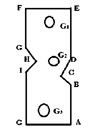
Рис. 1. Область S

Fig. 1. Region S

xy

Here n ₁, n ₂ – components of the outer normal vector to a piecewise smooth outer contour and hole contours bounding a finite region S . The region S . is shown in Fig. 1. X , Y - components of the external force vector.

Next, we assume that the material is in a plastic state on the lateral surface and the contours of the round holes, so the von Mises relation is included in (3). Here k is the plasticity constant, equal to the yield strength under pure shear.

We assume that the strip is stretched by efforts сту|у=I = 2k, сту|у=-1 = -2k,                          (4)

and the remaining boundaries of the outer contour and holes are considered stress-free.

It follows:

- on the boundaries AB, DE from (3) we obtain ст _у = 2 k , ст _x = 0, т = 0.

- on the boundaries FG, IJ - ст _у = - 2 k , ст _x = 0, т = 0. поставить зпт

- on the boundaries CB, GH and the boundaries r i - ст _у = 2 kn 1 ², ст _x = 2 kn 2 , т = - 2 kn 1 n ₂.

- on the boundaries CD, HI ст _у = - 2 kn 2 , ст _x = - 2 kn 2 , т = 2 kn 1 n ₂.

We will look for a solution to problems (1) – (3) in two stages. At the first stage, the Dirichlet prob lem for the Laplace equation Аp = 0 is solved, where ст X +ст у = p ( x, у ).

From (3) we obtain p = 2 k       on   DEFGH and ri p = -2 k      on HIJAB.

Standard methods are used to solve this problem. As a result, the function p ( x , y ). is found in the region S

At the second stage we solve the problem

^ст ^ ₊ «L ₌ 0, ^-^ x . ₊ S p = 0,     Убрать зпт                    (8)

дx ду      дx   ду   ду with the following boundary conditions, which follow from (3):

• -    on the boundaries DE, FG, IJ, AB ст x = 0, т = 0. ЗПТ

• -    on the boundaries CD, GH и Г_i             ст x = 2 kn 2 , т = - 2 kn 1 n ₂.                           (9)

• -    on the boundaries BC, IH          ст x = - 2 kn 2 , т = 2 kn 1 n ₂.

For convenience, we write equations (8) in the form

Л = U x + V y = 0, F 2 =- U y + V x + f = 0,                        (10)

dp where стx = u, т = v,— = f, further, the index below will indicate the derivative with respect to the dy corresponding argument.

For convenience, we will rewrite the boundary conditions in new terms.

On the boundaries DE, FG, IJ, AB u = 0, v = 0.

On the boundaries CD, GH и r i u = 2 kn 2 , v = - 2 kn 1 n ₂.                                     (11)

On the boundaries BC, IH u = - 2 kn 2 , v = 2 kn 1 n 2 .

Let us solve the boundary value problem (10), (11) using conservation laws.

Conservation laws of a system of equations (10)

Definition. The conservation law for the system of equations (10) is an expression of the form

A x + B y =® i F i -м 2 F 2 ,                                 (12)

where м 1 , м 2 - linear differential operators that are not simultaneously identically equal to zero, A = a 1 u + P 1 v -у ¹, B = a ² u + p ² v + у ²,                           (13)

a ¹, p ¹, у ¹, a ², p ², у ² - some smooth functions depending only on x , y .

Comment. A more general definition of the conservation law, suitable for arbitrary systems of equations, can be found in [16].

From (12) taking into account (13) we obtain a1 u + a1 ux + p1 Yv + p1 vY + у' + a2 u + a2 uv + p2 v + p2 vv + у2 = x    x x    x x y    yy    yy

= M1( ux + vy) + W2<-uy + vx + f) = 0.(14)

From (14) it follows ax + ay = 0, px + py = 0, a1 =ro1,p1 = м2, a2 = -м2,р2 = м1, уX +у 2 = м2 f.

From this we get a1 =p2, a2 =-p1.(15)

That's why ax-py = 0, ay + px = 0.(16)

From the given formulas it follows that the system of equations (10) allows for an infinite number of conservation laws; below only those will be given that allow us to solve the problem.

Since the conserved current has the form

A = a ¹ u + p ¹ v - у ¹, B = -p ¹ u + a ¹ v + у ².

From (16) using Green's formula we obtain

JJ ( A _x + B _y ) dxdy = J - Ady + Bdx + ^ J - Ady + Bdx = 0,                (17)

S                       L                    i Гi where S – region, limited by the curve L and the contours Гi.

Solution of the problem (10), (11)

To find values inside the region S , it is necessary to construct solutions of the Cauchy–Riemann system (16) that have singularities at an arbitrary point ( x 0 , y 0 ) e S .

The first of these solutions is

a1

x - x0

⁽ x - x 0 ) 2 + ^{( y} - ^y 0 ) 2

, P 1 =------ У-y -----2 , Y ¹ = f------ У-y -----г fdx , 1 2 = 0. (18)

(x - xo)2 +(y - yo)2       J(x - xo)2 +(y - yo)2

At the point ( x 0 , y 0 ) e S functions a ¹, p ¹ have singularities, so we will surround this point with a circle

• e : ( x - x o ) ² + ( y - y о ) ² = e ².

Then from formula (17) we obtain

E

i

f - Ady + Bdx + f - Ady + Bdx + f - Ady + Bdx = 0,

Г i

L                  e

Let us calculate the last integral in formula (19). We have

- Ady + Bdx = f-(-----u (x - x0)    2--v(y - y0)    2 +/) dy + e (x-x0)2+(x-x0)2 (x-x0)2+(x-x0)2

+

-      u ( y ^- y 0 )

у ( x - x o ) 2 + ( y - y o ) 2

______v ⁽ x - ^x 0 )______

(x - xo)2 + (y - yo)2 J

Let's enter new coordinates x - x ₀ = e cos ф , y - y ₀ = e sin ф , we gain

2n f-Ady + Bdx = f [-(ucosф + vsinф)cosф-(usinф + vcosф)5inф]dф = e0

2n f udф = -2пu (x0, y0).

The last equality is obtained by the mean value theorem e ^ 0.

To finally construct the solution, we find the values u , v on the boundary L . From formulas (15) we obtain

2 no _x ( x ₀, y ₀) = f у ¹ dy + f - ( - 2 kn 2 a ¹ + 2 kn 1 n ₂ p 1 + Y 1 ) dy + (2 kn 2 p 1 + 2 kn 1 n 2 a ¹) dx + AB BC

• - f (2 kn 2 a ¹ - 2 kn 1 n ₂ p 1 + 1 1 ) dy + (2 kn 2 p 1 + 2 kn 1 n 2 a ¹) dx - f у ¹ dy - f у ¹ dy + f у ¹ dy + CD                                               DE EF FG

+ f - (2 kn 2 a ¹ - 2 kn 1 n ₂ p 1 +у 1 ) dy - (2 kn 2 p 1 + 2 kn 1 n 2 a ¹) dx +

GH

+ f - ( - 2 kn 2 a ¹ + 2 kn 1 n ₂ p 1 - у ¹) dy + (2 kn 2 p 1 + 2 kn 1 n 2 a ¹) dx + f у ¹ dy - f у ¹ dy + HI                                                                     IJ JA

+ E f (2 kn 2 a ¹ - 2 knn ₂ p 1 + у ¹) dy + (2 kn 2 p 1 + 2 kn 1 n 2 a ¹) dx . i Г i

We take the second solution of the system of equations (16) in the form n 1 _       y - y 0         R1 _      X - x0

a              7              7 , P                7              7,

( x - x 0 ) + ⁽ y - y 0 )           ⁽ x - x 0 ) + ⁽ y - y 0 )

7 1 = - j 7------ x 'x 7 fdx , ^{7 2} = 0-                           (22)

( x - x ₀ ) + ( y - y ₀ )

Having carried out calculations similar to those carried out with solution (18), we obtain

2 пт (x ₀, y ₀) = j у ¹ dy + j - ( - 2 kn 2 a ¹ + 2 kn 1 n ₂ p 1 + 7 ¹) dy + (2 kn 2 p 1 + 2 kn 1 n 2 a ¹) dx + AB BC

• - j (2 kn 2 a ¹ - 2 knn ₂ p 1 + y 1 ) dy + (2 kn 2 p 1 + 2 kn 1 n 2 a ¹) dx - j 7 ¹ dy - j 7 ¹ dy + j 7 ¹ dy CD                                               DE EF FG

+ j - (2 kn 2 a ¹ - 2 kn 1 n ₂ p 1 + 7 ¹) dy - (2 kn 2 p 1 + 2 kn 1 n 2 a ¹) dx +

GH

+ j - ( - 2 kn 2 a ¹ + 2 kn 1 n ₂ p 1 - 7 ¹) dy + (2 kn 2 p 1 + 2 kn 1 n 2 a ¹) dx + j 7 ¹ dy - j 7 ¹ dy + HI                                                                     IJ JA

+ ^ j (2 kn 2 a ¹ - 2 kn 1 n ₂ p 1 + 7 ¹) dy + (2 kn 2 p 1 + 2 kn 1 n 2 a ¹) dx .                  (23)

i Г i

Conclusion

The paper proposes a method for solving a boundary value problem describing the elastic-plastic stress state of a strip with side cuts and holes. In this case, stress calculations a _x , т are reduced to calculating contour integrals along the boundaries of the region, and the stress a _y is determined from the solution of problem (11), (12) by numerically solving the Dirichlet problem for the Laplace equation. After determining all the components of the stress tensor, it is necessary to find the points of region S at which the yield strength is reached. This allows us to construct an elastic-plastic boundary and thereby estimate the strength of the plate under consideration. Currently, a program is being developed that allows us to construct an elastic-plastic boundary for stretchable plates with cuts and holes.