Some interrelations between quantum feedback control theory, quantum filtering and quantum information processing. Pt 1

The advent of quantum information theory and the ever-increasing experimental possibilities to implement this theory on real physical systems has created great demand for a theory on the control of quantum systems [1-12]. Since qubits (i.e., two-level quantum systems) make up the hardware (HW) for quantum information processing one important question is how to optimally control or engineer their states. Many problems of quantum computation and nanotechnologies can be formulated in terms of quantum optimal control of unitary or decohering gates [8-18]. Most previous work on the optimal control of qubit states uses an open loop strategy with a variational calculus approach to optimization [17-22]. However, in order to apply controls one must consider the qubit as an open quantum system which gives the possibility for time-continuous non-demolition measurements and thus a closed (feedback) loop strategy would be more advantageous. A feedback strategy we employed using dynamic programming which is a globally optimal solution to the control problem and thus extends the previous locally optimal variational approaches [17, 18].

Related works . Feedback control was introduced into quantum dynamics in the early 1980’s, but it was not until the 1990’s that it began to be studied and applied in earnest. A mathematical theory of feedback control in quantum systems was introduced by Belavkin, who obtained a quantum version of the Stratono-vich equation, which is the classical equation to describe the continuous measurement of a system. The Kalman-Bucy filter is the special case of the Stratonovich equation for linear systems, in which the measurement is restricted to linear functions of the dynamical variables. Belavkin’ s work prevented it from having an impact in the physics community, and the quantum version of the Stratonovich equation, referred to as the Stochastic Master Equation (SME), was obtained independently by Wiseman and Milburn building on the work by Carmichael. Srinivas and Davies, Gisin, and Diosi also presented stochastic equations for measured systems in this time period. In 1994, Wiseman and Milburn showed that a Markovian master equation could be derived to describe continuous feedback in quantum systems, called Markovian feedback , if the feedback was given by a particularly simple function of the stream of measurement results. In 1998, Yani-gasawa and Kimura and Doherty and Jacobs introduced the notion of performing feedback using estimates obtained from the SME, in the control literature and physics literature, respectively. Both sets of authors showed that for linear systems this class of feedback protocols was equivalent to modern classical feedback control, so that standard results for optimal control could be transferred to quantum systems. This method was in fact that proposed by Belavkin in 1983 in analogy to that used in classical control theory. In quantum control, using estimates obtained from the SME is often referred to as Bayesian feedback to distinguish it from Markovian feedback. In the former the measurement results are processed (“filtered”) to obtain an estimate of properties of the current state, whereas in the latter the measurement stream is fed back directly [11].

Remark . Wiseman showed that feedback mediated by continuous measurements can in fact be implemented without measurements [16]. To see how this works, let us consider two parallel mirrors between which a single mode of the electromagnetic field is trapped (the two mirrors are referred to as an “optical cavity”). The light that leaks out through one of the mirrors can be detected, and the information is used to manipulate the optical mode. Alternatively, the output light can be directed to a mirror of another optical cavity, and thus forms an input for this cavity. If we then connect an output from the second cavity back to the first we have a loop, and light can be made to travel only one way around the loop by the use of optical circulators. For describing this situation the quantum input-output theory developed by Collet and Gardiner is invaluable. The process of connecting quantum systems together via free-space one-way traveling-wave fields was first considered by Gardiner and Carmichael, where the former called it a “cascade connection”. Wiseman showed that cascade connections can implement the same feedback control processes as Markovian measurement-based feedback and can perform tasks that the latter cannot.

A second notion of feedback control without explicit measurements was introduced by Lloyd in 2000. He suggested that a unitary interaction between two quantum systems could be used to implement feedback control. This can be achieved, for example, by choosing the interaction so as to correlate the two systems, i.e., the controlled system and the controller, whereby the state of the controller is dependent on the state of the system. One then chooses a second interaction in which the evolution of the system depends on the state of the controller. This particular process is equivalent to a measurement followed by a unitary feedback operation that depends upon the measurement result, although coherent feedback processes are not restricted 3

to this form. Both kinds of “measurement-free” feedback, that mediated by cascade connections and that which uses unitary interactions are now referred to as coherent feedback control (CFC), and the latter is often called “direct” coherent-feedback. All control involving explicit measurements is usually called measurement-based feedback control, or just measurement feedback control (MFC) [1-27].

In the 2000’s James and his collaborators studied “feedback networks” of linear quantum systems connected by one-way fields , and Gough and James built on input-output theory to construct a compact and convenient formalism to handle arbitrarily complex networks. More recently a number of authors have considered the use of nonlinear coherent-feedback networks for various control tasks. In 2009, Nurdin, James, and Peterson showed that linear coherent feedback networks could out-perform linear measurementbased feedback, suggesting that measurement-based feedback was limited by the need to reduce the information about a system to classical numbers. It is also shown quite recently that coherent feedback can achieve more for generating quantum nonlinearity and cooling compared with the measurement-based feedback. The relationship between measurement-based and coherent feedback is a topic of current research.

Feedback control theory of open quantum systems

There are not only fundamental differences between measurement-based and coherent feedback, but also important practical differences. Making measurements on quantum systems, often possessing only a few quanta, usually requires a tremendous amplification of the signal. This is because the measurement results, by definition, are well-defined classical numbers. To robustly store and manipulate such numbers requires states with energies much greater than a single quantum. Amplifying signals at the single-quantum scale without swamping them with noise is a great challenge, and is one major practical disadvantage of measurement-based feedback. A second disadvantage is the timescale required to obtain and then process the measurement results (usually on a digital device).

On the other hand, measurement-based feedback has the advantage that the processing of the information is essentially noise-free. By contrast, if a quantum system is used as a controller it will likely be subject to noise processes from its environment. It may also be less clear how to use the quantum system to process the information to achieve a control objective. It is important to note that the method of “adaptive feedback”, in which the term “feedback” is used, is not the feedback control, i.e., measurement-based or coherent feedback that we are concerned with in this review. Adaptive feedback is a method for obtaining control protocols, not a class of protocols for controlling a system. In this method, one chooses an arbitrary control protocol, tries it out on the system, and based on the result make a modification to the protocol and tries it again. In this way one can use one of many search algorithms to look for a good protocol. Researchers who refer to adaptive feedback as a feedback method distinguish the feedback control we consider here by calling it “real-time (on-line) feedback control”.

Remark . It is also important to note that we do not discuss here all the ways in which feedback can be realized. One could, for example, perform a series of “single-shot” measurements with a discrete set of outcomes, and perform a unitary action on the system for each outcome. While there are certainly a range of interesting and non-trivial questions regarding such feedback, such as controlling thermal dynamics and quantum error correction, the mathematical machinery required to analyze it does not require stochastic differential equations. This is also true of coherent feedback implemented via unitary interactions. This latter topic has only recently begun to be explored in earnest, and there are certainly many open questions. However in this review we focus on continuous-time feedback control, both measurement-based and coherent. Both of these require the use of stochastic (Ito) calculus, something that is less familiar to many researchers in quantum theory. While measurement-based feedback requires only the usual Ito stochastic calculus, cascaded quantum feedback requires a quantum version of Ito calculus developed by Gardiner and Collett as part of their input-output theory. This quantum stochastic calculus was also developed independently by Hudson and Parthasarathy in a more rigorous measure-theoretic way. A readily accessible introduction to Ito calculus can be found in Appendices 1, 2 and 3, and the quantum version is described in [28-31].

To distinguish between experiments that realize quantum feedback control rather than classical control, we apply the criterion that an experiment involves the former if quantum measurement theory is required to correctly explain its results. This is certainly the case if the control process realizes a signature of quantum 4

behavior that is not manifest classically. For linear systems, the only distinction between quantum and classical motion is that the joint-uncertainty of position and momentum is limited by Heisenberg’s uncertainty principle. A measurement introduces noise because a reduction in the uncertainty of one canonical variable tends to increase the uncertainty of the conjugate variable. Feedback control of a quantum harmonic oscillator can thus be considered quantum mechanical if either (i) the “backaction” noise from the measurement must be taken into account in understanding the behavior, or (ii) alternatively one of the canonical variables has its uncertainty reduced below that of the vacuum state (so-called “squeezed states”).

Remark . Experiments implementing measurement-based feedback in the quantum regime were realized initially in quantum optics, where it first became possible to measure individual microscopic degrees of freedom with sufficient fidelity. These were followed by experiments involving trapped atoms and ions, and very recently it has become possible to realize measurement-based feedback control in mesoscopic superconducting circuits. Experiments involving continuous coherent feedback were performed prior to those realizing continuous measurement-based feedback, although at the time these experiments were not thought of as involving feedback. An example is the cooling of trapped ions using the “resolved sideband” cooling method.

Advances in feedback control of quantum open systems

The importance of feedback control theory in the control of open quantum systems was first recognized by V.P. Belavkin. As in the classical case with partially observer systems, a feedback control strategy is usually favorable to the open loop control (without feedback). Optimal feedback control strategies for the open quantum oscillator appeared even earlier and a quantum Bellman equation for optimal feedback control was introduced for a general diffusive and a counting measurement process. An interest in optimal quantum control and stability theory has recently emerged in the optics community. From a more formal perspective, one could say that quantum mechanics is believed to be a correct microscopic theory of (non-relativistic) physics but that the reduced dynamics of subsystems nearly always corresponds closely to models that fall within the domain of classical mechanics. Hence strongly non-classical behavior can only be observed in a subsystem on timescales that are short compared to those that characterize its couplings to its environment (see, Figures 1 and 2).

A quantum system is described by its corresponding Schrödinger’s equation. The Schrödinger’s equation for a quantum control system dw(x,t) r                                z x

----= |_ Hо (t, x ) + Ui (t) Hi (t, x )J w ( x, t), where H is the free Hamiltonian (energy) of the system; H is the interaction Hamiltonian of the system while being coupled to the control apparatus in the semiclassical treatment; w (x, t) is the state of the system. Open loop quantum control system is considered as a single larger system in an augmented state space “System + Environment = Hs ® Ил .” A quantum system interacting with a thermal bath is called an “open” quantum system.

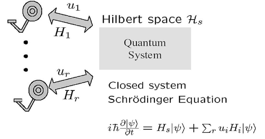
Figure 1. Closed quantum system

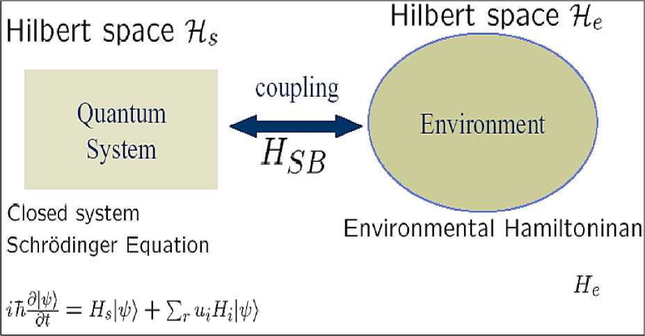
Figure 2. Open quantum system

Open quantum systems lose their coherence or superposition in the order of a few microseconds to milliseconds depending on the interaction. An open quantum system can be described as follows (see, Figure 3).

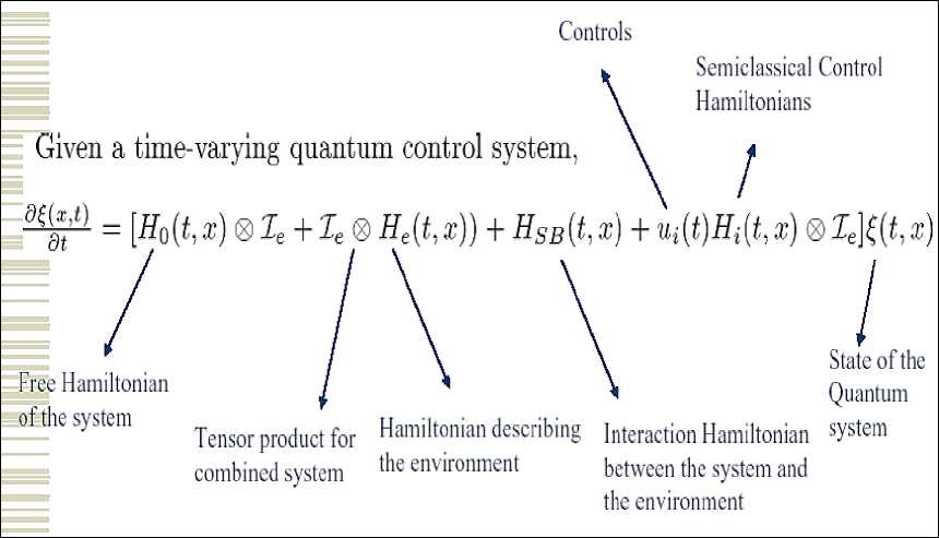
Figure 3. Structure of open quantum control system

Figure 4 show structure of quantum control systems for described cases.

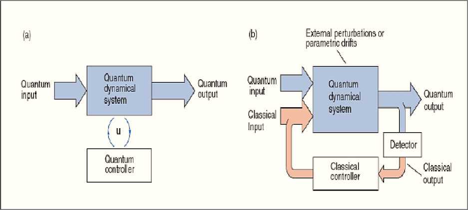
Figure 4. Structures of open-loop (a) and closed-loop (b) quantum control systems

Let us consider the example of another approach to quantum feedback design.

Coherent Quantum Feedback

As explained above, measurement-based feedback involves using the results of measurements on a quantum system to direct its motion. When we make a measurement on a quantum system, we obtain classical information. But we necessarily obtain only partial information about the dynamical variables, and in general we disturb the state at the same time. It is therefore interesting to consider a feedback loop in which classical information is not extracted. This concept, now referred to as coherent feedback, was first introduced by Lloyd in 2000, and it can be seen as the more general case of the all-optical feedback proposed earlier, in 1994, in quantum optical systems by Wiseman and Milburn. The idea is that instead of having a classical controller that makes a measurement on the system, the controller is a quantum system, and the control is achieved simply by having the two systems interact (see, Fig. 5).

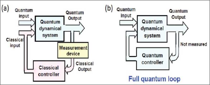
Figure 5: (Color online) Comparison of (a) measurement-based feedback and (b) coherent feedback. In measurement-based feedback in (a), the system (in blue) is controlled by a classical feedback loop (in pink); while in coherent feedback (b) the system is coherently controlled by a fully quantum feedback loop.

To understand this better, it is worth examining the Watt governor, which has a very simple feedback mechanism. The purpose of the Watt governor is to control the speed of an engine. To do this, the engine is connected to a simple mechanical device so that it spins the device. The device is designed so that the centrifugal force from the spinning causes it to expand, so that the faster the engine spins, the more it expands. This expansion is then used to reduce the fuel supply to the engine, thus stabilizing the engine at some chosen speed. The nice thing about this simple feedback system is that we can think of it as a loop in which the control device obtains information from the engine, and uses this to control it. It is also clear that the engine and controller are merely two coupled mechanical systems. In the Hamiltonian description of the joint system, there is therefore no loop, but merely an interaction between the two systems. A quantum controller can therefore act in the same way, performing feedback control even though the description of the system may not involve an explicit loop.

In fact, there is a way to make the loop explicit for a quantum controller in which there are no measurements. This is done by coupling the system to a travelling-wave electrical (optical) field that propagates in one direction from the system to the controller. We then use a second travelling-wave field that propagates from the controller to the system, thus closing the loop. To do this, the two travelling fields must continue propagating after they interact with the systems, and this introduces an irreversible element to the dynamics. However, since control systems are usually intended to introduce some kind of damping to the system, this irreversibility need not be detrimental. In what follows, we discuss feedback control that employs a unitary (Hamiltonian) interaction between the system and controller, often referred to as direct coherent feedback , where the interaction is mediated by travelling-wave fields, often referred to as field-mediated feedback.

The separation principle in open quantum control systems

In the case of any macroscopic object, such as an ordinary mechanical pendulum, there are so many such couplings (e.g. via mechanical coupling to its support and to air molecules) that these timescales are inaccessibly short. From an even more abstract perspective, one could say that Schrödinger’s equation is meant to apply to the universe as a whole (whose ‘internal’ degrees of freedom are densely interconnected) while physical experiments deal only with embedded subsystems. Unless great care is taken to suppress the environmental couplings of an experimental system, the overwhelming tendency is for its behavior to appear classical, or at least imperfectly quantum.

As was show, since we never have complete observability of quantum systems, the problem of quantum feedback control must involve a filtering procedure in order to measure and control the system optimally.

Figure 6 show the separation principle of open quantum control system.

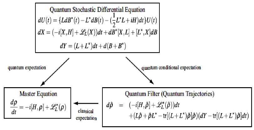
Figure 6. The separation principle in open quantum control systems

Measurement for a quantum system cannot be performed without probabilistic back-action. In general, the alteration of the system caused by the measurement is too drastic and instantaneous, and it prevents realtime feedback control. A possible way to avoid this difficulty is measuring the target quantum system indirectly in continuous time. This is the essential idea of continuous quantum measurement. It is realized by keeping the target quantum system interacting with another quantum system called probe system and measuring the probe system in continuous time. As the result, we obtain classical signal containing information of the target quantum system. We can use the signal to calculate the state of the target quantum system and utilize the calculated state to determine the control input. This is the basic idea of the measurement-based quantum feedback control and it is illustrated in Fig. 7.

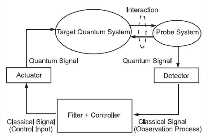
Figure 7. Conceptual diagram of the measurement-based quantum feedback control

This situation is analogous to that of the feedback control of partially observable classical stochastic systems. As in the classical case, filtering theory for quantum systems , i.e., quantum filtering theory provides a basis for feedback control of quantum systems under such a situation.

We can separate these two problems and consider first the problem of quantum filtering .

Advances in quantum filtering

In quantum filtering theory pioneered by Belavkin, the quantum filtering equation for the system with a chosen continuous non-demolition measurement (NDM) has to be derived. A system observed through its interaction with the electromagnetic field by continuous measurement of some field observables, needs to be updates continuously in time to incorporate the information gained by the measurement. That is we have to condition the quantum state of the system on the obtained measurement results continuously in time. The quantum filtering equation is a stochastic differential equation for the conditioned state in which the innovation process, representing the information gain, is one of the driving terms. In the quantum optics literature, some particular forms of the filtering equation were introduced in the 1990s as stochastic master equations (although without any reference to the original derivation). As in the optics literature, we take the filtering equation as our starting point; however, the driving Wiener process is not treated as the noise, but as an innovation process. For more background on the derivation of this stochastic equation as a general filtering equation in an open quantum system conditioned with respect to a non-demolition observation.

Once the quantum filtering equation is obtained, we are left with a classical control problem. In particular, if the state of a qubit is parameterized by its polarization vector in the Bloch sphere, i.e., a vector in the three-dimensional unit ball providing sufficient coordinates for the system, the filtering equation provides stochastic dynamics for the polarization vector. The control is present in the dynamics through Rabi oscillations, which perform rotations of the polarization vector in the Bloch sphere caused by a laser driving the qubit. The phase and intensity of the laser are the parameters that can be controlled.

The main aim of this article is to demonstrate the relevance of classical control and quantum filtering when controlling quantum systems. This is shown by the example of optimal control of a two-level quantum system. A cost function, which is a measure of optimality of the control, is introduced and the corresponding Bellman equations are derived for this system. From these equations, we produce an optimal control strategy which depends on the solutions to the corresponding Hamilton-Jacobi-Bellman equation. In general these solutions are very difficult to find, even numerically, so we resort to a physically motivated simplification of the dynamics by considering a qubit in a strongly driven, heavily damped, optical cavity. This enables us to present an exact solution to the control problem.

Quantum probability

Though they are both probabilistic theories, probability theory and quantum mechanics have historically developed along very different lines. Nonetheless the two theories are remarkably close, and indeed a rigorous development of quantum probability contains classical probability theory as a special case.

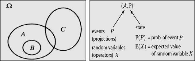
Figure 8 is demonstrated the definitions and differences in classical and quantum probabilities.

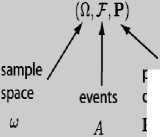
probability distribution

Р(Л) = prob, of event A E(JQ = expected value of random variable X

(a)

(b)

Figure 8. Classical (a) and quantum (b) probability definitions

Classical physics is built on foundations of classical logic, which is closely related to classical probability. We may think of quantum mechanics as the description of physical systems using a non-commutative 10

probability theory (quantum probability). In quantum probability theory states may be defined using states | ^ or density operators p as E [ X ] = ^| X |^ or E [ X ] = Tr [ p X ] . Algebras A of events describe information in both classical and quantum probability.

The simple example in Figure 9 depicts that when vectors are used to implement both events and densities the probability in the vector space is the squared inner product between the vectors, that is, the squared size of the projection of | A onto | ^ .

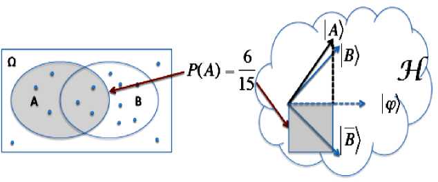
Figure 9. The correspondence between classical probability and quantum probability

The embedding of classical into quantum probability has a natural interpretation that is central to the idea of a quantum measurement: any set of commuting quantum observables can be represented as random variables on some probability space, and conversely any set of random variables can be encoded as commuting observables in a quantum model.

Thus in the classical probabilistic model, events (e.g., word occurrences, category memberships, relevance, location, task, genre) are represented as sets and the probability measure is based on a set measure, e.g., set cardinality. In contrast, in quantum probability, events are represented as orthonormal vectors and the probability measure is the trace of the product between a density matrix and the matrix representing an event as summarized in Table 1.

Table 1. The correspondence between classical probability and quantum probability

Notion	Classical	Quantum
Event space Random event Probability Measure	12 Set Set measure	Hilbert vector space 'AY Orthonormal basis {|S), |S)} State vector |y?)

The quantum probability model then describes the statistics of any set of measurements that we are allowed to make, whereas the sets of random variables obtained from commuting observables described measurements that can be performed in a single realization of an experiment. As we are not allowed to make noncommuting observations in a single realization, any quantum measurement yields even in principle only partial information about the system.

Quantum control with learning loop

The situation in quantum feedback control is thus very close to classical stochastic control with partial observations. A typical general (with learning loop) quantum control scenario, representative of experiments in quantum optics, is shown in Figure 10.

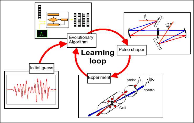
Figure 10. A closed-loop process for teaching a laser to control quantum systems [The loop is entered with either an initial design estimate or even a random field in some cases. A current laser control field design is created with a pulse shaper and then applied to the sample. The action of the control is assessed, and the results are fed to a learning algorithm to suggest an improved field design for repeated excursions around the loop until the objective is satisfactorily achieved]

The components of a learning-loop can look very different depending on the specific application. In abstract terms a learning-loop consists of an action under external control which acts on a system and produces there a system response. Due to the natural correlation between action and response an algorithm can be used to learn how to change the action to control the response in a desired fashion.

Remark . In the coherent control experiments as already pointed out the controlled action are the tailored femtosecond (fs) laser pulses. The external control knobs are all integrated in a single pulse shaping device. The system response is the feedback signal retrieved from experiment. It is feuded into the optimization algorithm that accordingly steers the pulse shaper to improve the laser pulse shape. The time for the learningloop to provide an optimal pulse is given by the total number of iterations multiplied by the time it takes to perform one iteration. This time is given by the response time of each of the elements that constitute a closed-loop experiment: laser repetition rate, pulse shaper, learning algorithm and feedback signal retrieved from experiment. Hence it is not possible to be specific, so the total optimization time can range between a few minutes and several hours. In the following a more detailed description of a tailored pulse, its characterization and the feedback algorithm is discussed. This article concludes with a practical application of the learning-loop approach: the compression of fs-laser pulses to their bandwidth limit.

Remark. A mentioned above, no quantum measurement can give full information on the state of a quantum system; hence any quantum feedback control problem is necessarily one will partial observations, and can generally be converted into a completely observed control problem for an appropriate quantum filter as in classical stochastic control theory. Here we study the properties of controlled quantum filtering equations as classical stochastic differential equations (see above mentioned Figure 5). We then discuss methods, using a combination of geometric control and classical probabilistic techniques, for global feedback stabilization of a class of quantum filters around a particular eigenstate of the measurement operator.

We wish to control the state of a cloud of atoms, e.g., we could be interested in controlling their collective angular momentum. To observe the atoms, we scatter a laser probe field off the atoms and measure the scattered light using a homodyne detector (a cavity can be used to increase the interaction strength between the light and the atoms). The observation process is fed into a controller which cam feedback a control signal to the atoms thought some actuator, e.g., a time-varying magnetic field. The entire setup can be described by a Schrödinger equation for the atoms and the probe field, which takes the form of a “quantum stochastic differential equation” in a Markovian limit. The controller, however, only has access to the observations of 12

the probe. The laser probe itself contributes quantum fluctuations to the observations, hence the observation process can be considered as a noisy observation of an atomic variable.

As in classical stochastic control we can use the properties of the conditional expectation to convert the output feedback control problem into one with complete observations. The conditional expectation п ( X ) of an observable X given the observations { У : 0 <  s <  t } is the least mean square estimate of X_t (the observable X at time t ) given У . One can obtain a quantum filtering equation that propagates п ( X ) , or alternatively the conditional density matrix p defined by the relation п ( X ) = Tr [ p X ] • This is the quantum counterpart of the classical Kushner-Stratonovich equation (due to Belavkin) and plays an equivalent role in quantum stochastic control. In particular, as E [ X_t ] = E^ ( X ) we can control the expectations of observables by designing a state feedback control law based on the filter.

Remark . Note that as the observation process Y is measured in a single experimental realization, it is equivalent to a classical stochastic process (i.e. the observables Y commute with each other at different times). But as the filter depends only on the observations, it is thus equivalent to a classical stochastic equation; in fact, the filter can be expressed as a classical (Ito) stochastic differential equation for the conditional density matrix p . Hence ultimately any quantum control problem of this form is reduced to a classical stochastic control problem for the filter.

Problem : Case study will consider a class of quantum control problems of the following form. Rather than specifying a cost function to minimize, as in optimal control theory, we desire to asymptotically prepare a particular quantum state p in the sense that E [ X_t ] ^ Tr ^ p X J as t ^да for all X . As E [ X. ] ^ E ,( X ) • this comes down to finding a feedback control that will ensure the convergence P ^ p of the conditional density p . In addition to this convergence, we will show that controllers also render the filter stochastically stable around the target state, which suggests some degree of robustness to perturbations. We will discuss the preparation of states in a cloud of atoms where the z -component of the angular momentum has zero variance, whereas we will discuss the preparation of correlated states of two spins. Despite their relatively simple description the creation of such states is not simple.

Quantum feedback control may provide a desirable method to reliably prepare such states in practice (though other issues, e.g. the reduction of quantum filters for efficient real-time implementation, must be resolved before such schemes can be realized experimentally; we refer for a state-of-the-art experimental demonstration of a related quantum control scenario.)

Thought we have attempted to indicate the origin of the control problems studied here, a detailed treatment of either the physical or mathematical considerations behind our models is beyond the scope of this section; for a rigorous introduction to quantum probability and filtering we refer [11, 23-27]. Instead we will consider the quantum filtering equation as our starting point, and investigate the classical stochastic control problem of feedback stabilization of this equation. We first introduce some tools from stochastic stability theory and stochastic analysis that we will use in our proofs. We introduce the quantum filtering equation and study issues such as existence and uniqueness of solutions, continuity of the paths, etc. We pose the problem of stabilizing as angular momentum eigenstate and prove global stability under a particular control law. It is our expectation that these methods are sufficiently flexible to be applied to a wide class of quantum state preparation scenarios. As an example, we use the techniques developed above to stabilize particular entangled states of two spins.

Therefore when engineers set about to control a classical system with incomplete data, they can evoke the celebrated separation theorem which allows them to treat the problem of estimating the states of the system (based on typically partial observations) from the problem of how to optimally control the system (though feedback of these observations into the system dynamics). Remarkably, this approach may also be carried over to the quantum world which cannot be in principle completely observer: this was first pointed out by Belavkin.

Quantum measurement, by its very nature, leads always to partial information about a system in the sense that some quantities always remain uncertain, and due to this the measurement typically alters the prior to a posterior state in the process. The Belavkin non-demolition principle states that this state reduction can be effectively treated within a non-demolition scheme when measuring the system over time. Hence we may apply a quantum filter for either discrete or time-continuous non-demolition state estimation, and then consider feedback control based on the results of this filtering. The general theory of continuous-time nondemolition estimation derives for quantum posterior states a stochastic filtering evolution equation not only for diffusive but also for counting measurement; however we will consider here the special case of a Belavkin quantum state filtering equation based on a diffusion model described by a single white noise innovation.

We should also emphasize that the continuous-time filtering equation can be obtained as the limit of a discrete time state reduction based on von Neumann measurements; however this time-continuous limit goes beyond the standard von Neumann projection postulate, replacing it with a quantum filtering equation as a stochastic master equation. Once the filtered dynamics is known, the optimal feedback control of the system may then be formulated as a distinct problem. Modern experimental physics has opened up unprecedented opportunities to manipulate the quantum world, and feedback control has already been successfully implemented for real physical systems. Currently, these activities have attracted interest in related mathematical issues such as stability and observability.

The separation of the classical world from the quantum world is, of course, the most notoriously troublesome task faced in modern physics. At the very heart of this issue are the very different meanings we attach to the word state . What we want to exploit is the fact that the separation of the control from the filtering problem gives us just the required separation of classical form quantum features. By the quantum state we mean the von Neumann density matrix which yields all the (stochastic) information available about the system at the current time – this we also take to be state in the sense used in control engineering. All the quantum features are contained in this state, and the filtering equation it satisfies may then be understood as a classical stochastic differential equation which just happens to have solutions that are von Neumann densitymatrix-valued stochastic processes. The ensuing problem of determining optimal control may then be viewed as a classical problem, albeit on the unfamiliar state space of von Neumann density matrices rather than the Euclidean spaces to which we are usually accustomed. Once we get accustomed to this setting, the problem of dynamical programming, Bellman’s optimality principle etc. can be formulated in much the same spirit as before.

We shall consider optimization for cost functions that are non-linear functions of the state. Traditionally quantum control has been restricted to linear functions where – given the physical meaning attached to a quantum state – the cost functions are therefore expectations of certain observables. In this situation, which we consider as a special case, we see that the distinction between classical and quantum features may be blurred: that is, the classical information about the measurement observations can be incorporated as additional randomness into the quantum state. This is the likely reason that the separation does not seem to have been taken up before.

This basic fact of nature that at small scales – at the level of atoms and photons – observations are inherently probabilistic, as described by the theory of quantum mechanics. The traditional formulation of quantum mechanics is very different, however, from the way stochastic processes are modeled. The theory of quantum measurement is notoriously strange in that it does not allow all quantum observables to be measured simultaneously. As such there is yet much progress to be made in the extension of control theory, particularly feedback control, to the quantum domain.

One approach to quantum feedback control is to circumvent measurement entirely by directly feeding back the physical output from the system. For example, in quantum optics, where the system is observed by coupling it to a mode of the electromagnetic field, this corresponds to all-optical feedback. Though this is in many ways an attractive option it is clear that performing a measurement allows greater flexibility in the control design, enabling the use of sophisticated in-loop signal processing and non-optical feedback actua- tors. Moreover, it is known that some quantum states obtained by measurement are not easily prepared in other ways.

We take a different route to quantum feedback control, where measurements play a central role. The key to this approach is that quantum theory, despite its entirely different appearance, is in fact very closely related to Kolmogorov’s classical theory of probability is the fact that in quantum theory observables need not commute, which precludes their simultaneous measurement. Kolmogorov’s theory is not equipped to deal with such object: One can always obtain a joint probability distribution for random variables on a probability space, implying that the can be measured simultaneously. Formalizing these ideas leads naturally to the rich field of noncommutative or quantum probability . Classical probability is obtained as a special case if we consider only commuting observables.

Stochastic quantum control theory

Let us briefly recall the setting of stochastic control theory . The system dynamics and the observation process are usually described by stochastic differential equations of the Ito type. A generic approach to stochastic control separated the problem into two parts. First one constructs a filter which propagates our knowledge of the system state given all observations up to the current time. Then one finds a state feedback law to control the filtering equation. Stochastic control theory has traditionally focused on linear systems, where the optimal [linear quadratic Gaussian (LQG)] control problem can be solved explicitly.

A theory of quantum feedback control with measurement can now be developed simply by replacing each ingredient of stochastic control theory by its noncommutative counterpart. In this framework, the system and observations are described by quantum stochastic differential equation. The next step is to obtain quantum filtering equations. Remarkably, the filter is a classical Ito equation due to the fact that the output signal of a laboratory measuring device is a classical stochastic process. The remaining control problem now reduces to a problem of classical stochastic nonlinear control. As in the classical case, the optimal control problem can be solved explicitly for quantum systems with linear dynamics (see Figure 5).

The field of quantum stochastic control was pioneered by V.P. Belavkin in a remarkably series of papers in which the quantum counterparts of nonlinear filtering and LQG control were developed. The advantage of the quantum stochastic approach is that the details of quantum probability and measurement are hidden in a quantum filtering equation and we can concentrate our efforts on the classical control problem associated with this equation. Recently the quantum filtering problem was reconsidered by Bouten et al . and quantum optimal control has received dome attention in the physics literature.

The goal of this article is twofold. We review the basic ingredients of quantum stochastic control: Quantum probability, filtering, and the associated geometric structures. We then demonstrate the use of this framework in a nonlinear control problem. To this end, we study in detain an example directly related to any experimental apparatus. As this is not a linear system, the optimal control problem is intractable and we must resort to methods of stochastic nonlinear control, stochastic Lyapunov techniques to design stabilizing controllers us used, demonstrating the feasibility of such an approach.

Many results are motivated in studying the quantum control problem by recent development in experimental quantum optics. Technology has now matured to the point that state-of-the-art experiments can monitor and manipulate atomic and optical systems in real time at the quantum limit , i.e., the sources of extraneous noise are sufficiently suppressed that essentially all the noise is fundamental in nature. The experimental implementation of quantum control systems is thus within reach of current experiments, with important applications in, e.g., precision metrology and quantum computing. Further development of quantum control theory is an essential step in this direction.

Extension of control theory to the quantum domain has been a target of some researchers since the mid-1970a. The main motivation there was tied to the fact that measurements of any physical quantity inevitable disturbs the state of the quantum system The formulation of feedback control under this circumstance seemed to be a great challenge for control theorists. On the other hand, variational principle used in the optimal control manifests itself more explicitly in quantum mechanics, because its fundamental governing equation is energy preserving. This is perhaps another reason why quantum theory attracts control theorists.

Remark . In the early 1980a, more realistic pictures were brought forward in the field by a group of chemists who tried to control chemical reactions by properly arranging electromagnetic fields. They purpose was to increase the probability of favorable chemical reaction by means of adjusting the phase difference between two electromagnetic fields created by laser beams. Theoretical, as well as experimental, verifications of the possibility of materializing these attempts have been reported extensively in the literature of photochemistry. In these papers by chemists, control is ascribed to the selection of Hamiltonian due to the method of “ inverse problem ,” and is therefore essentially a feedforward control, as Gordon and Rice properly described. The chemical experiments on the reaction between the electromagnetic field and two or three level atomic systems led t one possible generalization of control theoretical notions, such as controllability. Since the evolution of a quantum system is given by the unitary operators with continuous parameters, the generalization is based on the unitary representation of Lie groups. This technique has resolved the quantum problem. The first theoretical work on feedback for quantum systems appeared in quantum optics, which treated the fluctuations of the photocurrent in a quantum mechanical way. The scholastic Schrödinger equation was first introduced in the early 1990s. This formulation enables one to control quantum systems via measurements, in which the quantum system is driven by interactions conditioned by the measurement outcomes. A definite class of states, referred to as Gaussian, is of particular interest is not only classical but also in quantum case. As a result, feedback control for the state via measurement was studied.

Recent progress in quantum electronics has opened up the possibility of quantum information technologies, which are expected to eliminate the bottlenecks of modern communication and computation. They are based on the notion of entanglement which is thought of as a quantum information resource. Entanglement is a quantum mechanical correlation which is produced only by nonlocal quantum mechanical interactions. In theoretical works, it is assumed that we can specify the quantum state at our disposal whenever we need it, no matter how the environment of the system would be. In other words, it is presumed that the quantum state can be controlled for the use of communication and computation. This presumption is far from trivial taking into account the fact that the quantum systems sometimes entangle with undesirable systems, which results in a noisy information resource, and consequently, it has been necessary to consider the production of entanglement in the light of quantum control accordingly. Feedback is a method whereby the performance and robustness of the system can be improved considerably, even if the system includes some uncertainty in its environment to which the system is highly structured. This article is devoted to the formulation of quantum mechanical feedback, in order to introduce the concepts and tools of control theory to quantum theory for understanding quantum systems and developing quantum control.

For a system placed among a large number of degrees of freedom interacting with one another, one may ignore the detailed dynamics of the external degrees of freedom by treating them statistically. If the system is weakly coupled to the external field is characterized by the singular correlation of the field. This singularity constitutes the description of the system though the stochastic differential equation or the forward Fokker-Plank-Kolmogorov equation. In the quantum case, in order to deal with quantum systems properly, physical variables should be quantized through the canonical commutation relation, which is essentially singular. An analogy between the singularities of the classical correlation function and the quantized commutation relation leads to a generalization of the stochastic differential equation subject to the quantum mechanical law.

There is a dual relationship in the description of quantum dynamics analogous to a one-to-one correspondence between the Fokker-Planck Kolmogorov equation and the stochastic differential equation. The former describes the evolution of probability distribution of the system which interacts with the external field. The influence of the external filed is not explicitly represented in this description because the information of the external field is averaged out. The latter is a dual description in the sense that it represents the evolution of physical variables, and the single path of the system along with the external filed is explicitly presented. Both are basically equivalent, however the latter provides the input-output relation of the system by which we can consider various connections of systems. If quantum systems are connected in a complex way, it is sometimes hard to derive the Hamiltonian which describes the behavior of the entire system because the connected systems are entangled with each other through the inputs/outputs, and consequently, the total Hamiltonian is not given by the sum of local Hamiltonians describing each component system.

Furthermore, the noncommutativity of quantum variables complicated the difficulty of the description of the filed, after having interacted with the system at some time then interacts with it again at some later time through a closed loop. This is why there has been little work on using nonclassical field to construct large quantum systems including closed loops. This article proposed a systematic procedure to obtain the Hamiltonian and the quantum stochastic differential equation that lead to a natural extension of control theory and some applications of quantum control. We will derive general dynamics of quantum feedback systems, based on the framework of quantum feedback systems, the application of quantum feedback to some of the most important problems in quantum theory are described.

We start with review which is a brief review of fundamental notions of quantum theory for introducing control theoretical viewpoints to quantum systems. In particular, it focuses on introducing the interaction between a system and environments in a quantum mechanical manner, because system control is essentially based on the plant-controller interaction. We introduce a quantum stochastic process as a noncommutative analog of Wiener process, in which the quantized electromagnetic field traveling in free space is the non-commutative input source (see, Appendices 1.2 and 3). An optical system is treated in terms of an idealized class of Hamiltonians describing a linear coupling of a localized system to the noncommutative input. The system then obeys the quantum stochastic differential equation which arises due to the stochastic nature of the noncommutative input operators. Then we deal with the quantum mechanical feedback in the proper context of quantum feedback system. The feedback connection of quantum systems has a wide range of applications that enables us to derive Hamiltonians for the applications for deriving the evolution of quantum systems connected in a complex way.

Quantum systems are in some ways closely analogous to classical ones, and in other ways quite distinct. An essential difference between them is that canonical observables are represented by noncommutative operators in quantum mechanics, whereas the corresponding classical variables are represented by scalar. The noncommutativity of observables leads to a significant departure from classical mechanics, known as the uncertainty principle , which states that no action can be done without introducing inevitable disturbances to quantum systems. Although certain uncertainties of physical variables could be also found in classical systems, it is remarkable in combination with another significant property: entanglement . These features cast light on the possibility of quantum information technologies and broaden the applications of engineering. In quantum cryptography, for example, spatially separated systems utilize entanglement for sharing keys, and the uncertainty principle guarantees that they can detect other observers trying to eavesdrop on the quantum key distribution.

Quantum control is recognized as an indispensable technology to provide the cannel resource needed for the communication between sender and receiver. The concepts and tools of control theory contribute not only to the understanding of dynamics of complex quantum networks, but also to the designing of the system for any purpose. An extension f control theory to the quantum domain enables us to deal with complex quantum systems in a systematic way.

A feedback system is, in general, supposed to consist of processes of obtaining information about the plant, processing it through a controller and changing the behavior of the system according to the output of the controller. The performance of the feedback system depends on the structure of the additional; degrees of freedom resulting from these processes. One possible method of constructing the auxiliary degrees of freedom is to utilize a measurement for obtaining the information about the plant and to process the measurement outcomes with a classical dynamics is that inevitable changes occur when the information from the measurements is read in macroscopic ways. This leads to a limitation on the performance of quantum feedback. The feedback process, however, need not necessarily be macroscopic and classical in practice.

An alternative method for quantum feedback control can be constructed in a completely quantum mechanical way, in which the entire processes of feedback is implemented by quantum systems. We discussed the dynamics of a cavity coupling to the electromagnetic filed traveling in free space. A cavity is thought of as a first-order quantum system driven by a stochastic field, sent through a quantum channel that entangles with the state of the system and produces the output. This characteristic allows us to have access to the system through the output signals in order to get the information about the system and to alter its behavior.

It has introduced the symmetric operator-ordering scheme (SOS) for defining the Hamiltonian of quantum networks, in which spatially separated systems interact with each other though the feedback and cascade connections. In this case, the dynamics of the system cannot be derived from the local Hamiltonian of each system in general, because of entanglement that is generated through the external field. According to SOS, we can obtain the Hamiltonian which explicitly shows the interaction between the component systems, and derive the evolution. In particular, when the input and the output of the system are of interest, it is described by a transfer function, which enables us to deal with complex quantum systems in a simple way. It is received wisdom that, in order to control the system, it is necessary to argument degrees of freedom of the system by connecting additional systems through the input-output. The quantum stochastic differential equation is available for the construction of the auxiliary degrees of freedom with the tools of control problems of quantum theory are reduced to conventional problems of control theory based of the developed formalism.

Models of quantum feedback control

In present issue we are discussed different models of quantum feedback control. Let us briefly describe here the applications of feedback control in quantum systems. We explain how feedback in quantum systems differs from that in traditional classical systems, and how in certain cases the results from modern optimal control theory can be applied directly to quantum systems. In addition to noise reduction and stabilization, an important application of feedback in quantum systems is adaptive measurement, and we discuss the various applications of adaptive measurements. We finish by describing specific examples of the application of feedback control to cooling and state-preparation in nano-electro-mechanical systems (NEMS) and single trapped atoms.

We study Quantum Control (QC) methods and its interrelations with advanced control. In particular, we are describing methods to control quantum systems in the arena of quantum and atomic optics, and quantum nanomechanics. The objective of QC is to determine which final (or target ) states of a quantum system are dynamically reachable from a given initial state. This is operationally achieved by applying to the system a sequence of simple control pulses.

Lately, various aspects of QC have been discussed in the literature, including the question of controllability of systems with continuous spectra, wave function controllability for bilinear systems, controllability of distributed systems, of molecular systems, of spin systems, of quantum evolution in NMR spectroscopy, and QC on compact Lie groups etc.

QC (same as quantum tomography) can be viewed as reciprocal aspects of the analysis of the states of a system. Both are connected to the problem of extracting the maximum amount of information from that system. In general, for quantum systems possessing a certain group of dynamical Lie-type symmetry, it has been shown, that the degree of controllability depends on the structure of a given Lie group.

Let us consider briefly the main idea of QC.

Some basic concepts of quantum control

A quantum system is said to be completely controllable if, given any two states | Vo ),|Vi) (we will restricted ourselves to pure states) there exists a time T >  0 and a set of admissible control functions [ ^f ( t ) ,-•, ^fM ( t ) ] defined for 0 <  t <  T , so that U ( 0 )| v₀) = | Vo)and U ( T ) | Vo) = I Vi) , where U ( t) is the evolution operator of the system.

Thus the objectives of quantum control are to find ways to manipulate the time evolution of a quantum system such as to

• o    Drive an initial given state to a pre-determined final state, the target state ;

or

• o    Optimize the expectation value of a target observable .

When a quantum system is invariant under the action of a (Lie-type) group of dynamical symmetry, the control functions are usually chosen so that the evolution operator is expressed as a product of some “elementary” group transformations, each representing a sequence of isolated physical “pulses”. The key is whether or not the control parameters lead to an evolution operator that is a generic element of the group. When this is the case, it has been shown that the system is completely controllable.

If, on the other hand, the evolution operator is not a generic element of the group but is an element of a subgroup of the dynamical symmetry group, the system is only partially controllable . The problem then consists in classifying families of states of the form: |y( t )^ = U ( t )| y₀) , i.e. families of states invariant under the action of the evolution operator. In other words, the problem consists in classifying the orbits of a subgroup, formed by all admissible evolution operators, in the Hilbert space of a given quantum system.

Example . As a simple example, let us start by reviewing how the controllability of a single two-level atom can be implemented by means of applying pulses of an external field. This is the simplest system, with SU ( 2 ) as the group of dynamical symmetry. In the rotating frame, the Hamiltonian for such a system

A reduces to H.t = — a + g (a + a ) in          z       \  +      — /

where A = ш_й — m^ is the external field frequency and a_{z ±} are the

Pauli matrices ( g is chosen real for simplicity). The frequency of the external field m^ is an adjustable parameter, so that two types of pulses can be applied to the atom: a resonant pulse, for which A = 0, leads to an evolution of the form R ( 0 ) , where R ( 0 ) is given below, and a dispersive pulse, for which AD g and which produces an evolution of the form D ( y ) , where D ( y ) is described also below. An evolution can then be obtained by patching together dispersive and resonant pulses to obtain the three-parameter transformation:

U (y, 0, ф) = D (y) R (0) D (ф), л cos 0

, i sin 0

i sin 0^Л cos 0_V

where 0 = gt 2 , y = —^ , ф = — -1 , D ( y ) = diag ( e^{l y} , e" i ^y) , R ( 0 ) =

Here, t , j = 1,2,3 , denotes the length of the intervals during which the appropriate pulse is applied.

The evolution operator U ( y , 0 , ф ) has a form of a generic element of SU ( 2 ) , the orbits of which form a three-dimensional sphere. The space SU ( 2 ) / U ( 1 ) □ CP¹ of all physically distinguishable states of a two-level atom contains a single orbit, so we immediately arrive at the conclusion that a single two-level atoms is completely controllable, i.e. for arbitrary |y₀) and |y( T )^ there exists U ( y , 0 , ф ) so that

I y(T )) = U (y( t3 ), 0( t2 ), ф( t1 ))|Уо> , where T = tx +12 +13.

We study the feedback methods of advanced control and rather than controlling, say, a jet engine, we can use feedback to control an object as small as a single atom. Feedback has many interesting and useful properties. It makes it possible to design precise systems from imprecise components and to make physical variables in a system change in a prescribed fashion. An unstable system can be stabilized using negative feedback and the effects of external disturbances can be reduced. Feedback also offers new degrees of freedom to a designer by exploiting sensing, actuation and computation. A consequence of the nice properties of feedback is that it has had major impact on man-made systems. Drastic improvements have been achieved when feedback has been applied to an area where it has not been used before.

The different stochastic equations correspond to different ways in which the system can be continuously monitored.

Quantum jumps

Consider the master equation

p=- i [ H, p]+1 Е (2 c^pc\ - cp c^p - рсц cp)                     (1)

² p

A stochastic equation that unravels this master equation, and that is driven by a point process, is d кс)

- iH +

1 Е( ^c.^ ⁽ t ) - ^c \ ^с р ) k) dt + Е

² p                              р

—1 | k c)^dN p

Here, for each μ , the increment dN is an increment of a point process, and takes only two values, either 0 or 1. The value 1 corresponds to an instantaneous event, and thus dN is equal to 1 only at a set of discrete points. The rest of the time dN = 0 . The events occur randomly and independently, and the probability per unit time that an event occurs for the process labelled by д is ^ c * c^ ^( t ) . This means that the probability for an event in the time interval [ t + dt ] is ^ c * c^ ^( t ) . The point-process increments satisfy the relations: E К dN p ( t ) ] = ( c p c p )( t ) , dN p dN . = dN p 8 p. .

Since Eq. (2) is a stochastic equation for the state vector, it is usually called a stochastic Schrödinger equation . We can alternatively write down a stochastic master equation for the density matrix P c = I k c) ^c I, which is

dPc = Е G L cp ]p.dNp (t) + H — iH — 1Е cP cp pcdt

p                      L

The superoperators Е G [ c_u p and H [ c ] p are defined as p

УG L cp ]Pc =  ^ tn — Pc ,  H [c ] Pc = cPc + Pcc — (c + c f) Pc p              Tr |cPccI

The point process (quantum jump) stochastic Schrödinger equation (SSE) describes, for example, an optical cavity in which the light that leaks out of the cavity is measured with a photon-counter. In this case there is a single Lindblad operator c = Y a^a , where / and a are the damping rate and annihilation operator for the cavity, respectively. The events at which dN = 1 correspond to the detection of a photon by the photo-detector.

More generally, a continuous measurement of the quantum variables A_t ( l = 1,..., m ) can be expressed as the stochastic master equation

m

dpc = -i [H, p] dt + Е (ГlD [Al ] Pcdt + TnlrZH [Al ] dW,)

Электронный журнал «Системный анализ в науке и образовании» and output equation dy, = (A) dt + . 1 dW (6) V 2^/ Г i where Fz and n represent the measurement strengths and measurement efficiencies.

The stochastic master equation (5) and the equation for the stream of measurement results, Eq. (6), can be derived from the quantum filtering equations. The quantum filtering equations give the evolution of the system and the output field before any measurement is made on the output field. Making a measurement on the output field turns the quantum filtering equations into a stochastic master equation. As mentioned above, we can simultaneously make more than one continuous measurement on a system, and we can simultaneously measure observables that do not commute. Since the respective dynamics induced by the continuous measurements of two different observables commute to first order in dt , we can think of the measurements of the two observables as being interleaved — the process alternates between infinitesimal measurements of each observable.

Note that a von Neumann measurement cannot simultaneously project a system onto the eigenstates of two non-commuting observables, but continuous measurements do not perform instantaneous projections. The effect of simultaneously measuring the position and momentum of a single particle is to feed noise into both observables. Measuring noncommuting observables therefore in general introduces more noise into a system than is necessary to obtain a given amount of information. The optical measurement techniques of heterodyne detection and eight-port homodyne detection are very similar to simultaneous measurements of momentum and position.

Markovian quantum feedback

The continuous collapse of the quantum state in continuous quantum measurement means that we can execute real-time quantum feedback control before the quantum state collapses to a completely classical state. That is the starting point of continuous measurement-based feedback control. This is the kind of feedback protocols and are now referred to as Markovian feedback. The reason for this name is that for this kind of feedback, if we average the evolution over all trajectories, the result is a Markovian master equation. This is not usually true for feedback protocols.

Let us consider a quantum continuous measurement of the operator A with efficiency η. From Eqs. (5) and (6), the measurement and output equations of this measurement can be expressed as dpc = -i [H, pc ] dt + FAD [ А] pcdt + ПГ^н H [ a ] PcdW(7)

and dy = (A) dt +  . 1 dW(8)

4 2'^nF A

These two equations can also be expressed equivalently by

Pc =- i [ H, Pc] + F A D [ A ] p,+ 4FvH H [ A ] p,s (t)

and

IA(t )=<А>+v^f; ^( *)

Электронный журнал «Системный анализ в науке и образовании» Выпуск №1, 2018 год where ^ ( t ) is the white noise satisfying E ( ^ ( t ) ) = 0, E ( ^ ( t ) ^ (t ‘ ) ) = 5 ( t — t ‘ ) . Formally, we can convert Eqs. (7) and (8) into Eqs. (9) and (10) by setting ^ (t ) = dW I dt .

The main object of measurement-based quantum feedback is to use the output signal I_A ( t ) to engineer the system dynamics given by Eq. (9). The most general form of the system dynamics, modified based on the output signal I_A ( t ) , can be expressed as

pf = F [ t, {IA (г) к e[0, t 1}] pf

where F^t, {IA (к) |r e [0, t]}j is the superoperator depending on the output signal IA (t) for all past times. In this general form of the response of the feedback control loop, the control induces both unitary dynamics and dissipation effects on the controlled system. However, for most of the existing studies, quantum feedback control is introduced coherently by varying the parameters in the system Hamiltonian, which leads to the following modified closed-loop stochastic master equation pf=—i H+H

( t ’ {I A (к) к e [ 0, t ]}) , Pf + Г A D [ A ] Pf + V^H [ A ] Pf% (t) .

As discussed above, in Markovian quantum feedback a term in the Hamiltonian is made proportional to the output signal. Denoting this term by Hy , we set H_f = I_A ( t ) F for some Hermitian operator F . Then, by averaging over the noise term and using the Ito rule of the white noise ^ ( t ) , we can derive the following Wiseman-Milburn master equation from Eq. (12):

p = -i [H, р] + ГAD [ A] p — i [F, Ap + pA] +1D [F] p .

П

The effects induced by the feedback loop are clearer in this form: (i) the first feedback term

— i [ F, A p + p A ] plays a positive role to steer the system dynamics to achieve the desired effects; and (ii)

the second feedback term — D [F] p represents the decoherence effects induced by feedback, which tends П to play a negative role for purposes of control.

The master equation (13) can be reexpressed as the traditional Lindblad form as following:

p = —i

H ₊ ( AF ₂- FA ) , p

+ D [ A — iF ] p + 1^ D [ F ] p .

Although the Markovian quantum feedback given by Eq. (13) is the simplest measurement-based quantum feedback approach, it can be used to solve various problems by choosing A and F appropriately. Markovian quantum feedback has been used to stabilize arbitrary one-qubit quantum states, manipulate quantum entanglement, generate and protect Schrödinger cat states, and induce optical, mechanical, and spin squeezing.

Bayesian quantum feedback

To make full use of the information provided by the measurement, we must process the measurement results using the SME (Eq. (5)) to obtain the conditional density matrix. Since this density matrix, along with the knowledge of the dynamics of the system, determines the probabilities of the results of any measurement on the system at any time in the future, any optimal strategy for controlling the system can ultimately be specified as a rule for choosing the Hamiltonian at time t as a function of the density matrix at that time and possibly the time itself: H (t) = f (p (t), t) . Feedback control in which the feedback protocol is specified in this way is sometimes referred to as “Bayesian feedback” because the SME is the quantum equivalent of processing the measurement record using Bayes’ theorem.

As we have mentioned above, the SME, since it requires simulating the full dynamics of the system, may be impractical to solve in real-time. Sometimes it is possible to approximately, or even exactly, reduce the computational overhead by choosing an ansatz for p that contains only a small number of parameters. The SME then reduces to a stochastic differential equation for these parameters. There is one class of systems in which an ansatz with a small number of parameters provides an exact solution to the SME, that of linear systems. A quantum system is referred to as linear if its Hamiltonian is no more than quadratic in the position and momentum operators, any Lindblad operators that describe the noise driving the system are linear in the position and momentum operators, and any measurements are (i) driven by Wiener noise, and (ii) of operators that are linear in the position and momentum.

The noise that drives linear systems reduces all initial states to Gaussian states (states that are Gaussian in the position and momentum bases, and thus have Gaussian Wigner functions), and Gaussian states remain Gaussian under the evolution. No proof of the first of these statements exists, but experience leads us to believe it. The second statement is not difficult to show, and implies immediately that if the state of a linear system is Gaussian, the SME reduces to a stochastic differential equation for the means and (co-)variances of the position and momentum. What is more, the dynamics of these variables are exactly reproduced by those of a classical linear system driven by Gaussian noise, and subjected to continuous measurements of the same observables. To correctly reproduce the quantum dynamics, for each continuous measurement made on the system a noise source must be added to the classical system to mimic Heisenberg’s uncertainty principle.

Example. Consider a linear quantum system with N degrees of freedom, and write the N position and momentum operators, denoted respectively by q and p , in the vector x = ( qv pv..., Qn , Pn )T

We scale these operators so that [qn, pn ] = i. If xm is the mth element of the vector x, then we have r      T                    N ( 01

[xn , xm ] = i2nm , where 2=® n=1 (-10

For linear quantum systems, the system Hamiltonian H and the dissipation operator L can be written as

Hs = |xTGx - xT2bu, L = ITx ,(16)

where G is a real and symmetric matrix, and b , l are real and complex vectors, respectively. The second term in H , including the time-dependent function u ( t ), describes the force applied by the feedback controller (see Fig. 11).

This feedback Hamiltonian must be linear in the conditional mean values of the position and momentum operators, in order to ensure that the system remains linear. This also means that there is a linear map from the measurement output Y to u ( t ), and thus a linear input-output relation for the controlled system. The dynamics of the controlled system can be expressed as the following linear quantum stochastic differential equation:

dx = Axdt + budt + i Jy’L [ IdB ^ - 1 * dB_in ] ,                        (17)

where the matrix A = S Г G + Im ( I * I T

The output equation (17) can be written as

dY ,.. = Fxd< + 4= ( dB n + <) •

V Y

F =I^T + 1^-

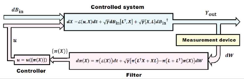
Figure 11: (Color online) Diagram for state-based quantum feedback. The controlled system (top branch, in blue) is described by a quantum stochastic differential equation driven by the quantum Wiener noise dB .

Part of the quantum output field Y from the controlled system is converted into a classical signal dW by a measurement device (shown in yellow) and then fed into the filter. The dynamics of the filter is determined by the quantum filtering equation driven by the classical Wiener noise, i.e., the innovation process dW. The estimated quantum state { п ( X ) } is fed into a classical controller to obtain a control signal u, which is then fed back to steer the dynamics of the controlled system. The filter and controller which form the classical control loop (in pink) can be realized by a classical Digital Signal Processor (DSP)

After quantum measurement, the dynamics of this linear quantum system can be fully described by the conditional means n (x) and variances Vart = P (P |Y), where Pt is the covariance matrix of the position and momentum variables with the (i, j) -element being P = ^-(AxiAxj + AxjAxz), and Axt = xt

^{- п} ( x i ) .

The conditional mean values π (x) obey the filtering equation dn(x) = An(x)dt + Budt + ^VartFT + ST Im(l)]x[dY-Fn(x)dt]           (19)

and the conditional covariance matrix satisfies the deterministic Riccati differential equation

Var_t = AVar, + VarA ^T + D-\_Var_tF ^T +S ^T Im ( l ) ]x[ FVar_t + Im ( l ^T ) s] ,          (20)

where D = S Re ( l*l ^T ) Z ^T . Thus, the filtering equation is equivalent to the closed set of filtering equations (19) for the first-order quadrature and the Riccati differential equation (20), which is finite-dimensional and thus simulated with relative ease. The quantum filter given by Eqs. (19) and (20) is called a quantum Kalman filter .

For linear quantum feedback control systems, many objectives, such as cooling and squeezing, can be reduced to the optimization of the following quadratic cost function of the system state x as

Ja = — xTSxT +—[ ГxTQx + uTRu 1

q 2 ^{T T} 2 o l ^r^ ^{т т т} ]

To obtain a closed-form control problem, we should first take the expectation value over the conditioned state and then average over all the stochastic trajectories to define a new quadratic cost function ^J = (^P ( ^J q t )) _c, where ^ c is the average taken over the classical Wiener noise dW . From Eq.(21) we have

1 ^T

~ ЦП ( xT ) Qn ( xT ) + Tr ( QVarT ) + uTRuT

d T + ( — n ( x_T ) S n ( x_T ) + — Tr ( SVar В (22) c 2                      2               c

Here the control u_t = u ( n ( x_t ) , Var_t ) is a function of the conditional means and variances n ( x_t ) and Var . The optimization of the quadratic cost function (22) subject to the quantum filtering equations (19) and (20) is a standard classical Linear-Quadratic-Gaussian (LQG) control problem which can be solved by the Kalman filtering theory well developed in the field of classical control.

Networks of quantum systems

The configuration of the feedback system in Fig. 5 has a unidirectional connection from the system to controller, which replaces the measurement in measurement-based feedback, but does not use a unidirectional coupling for the feedback part of the loop. We can, however, use a cascade connection for both, in which case we have a complete unidirectional loop. What we now need to know is how to describe these cascade connections mathematically. To do this, we use the input-output, or “quantum noise” formalism of Collet and Gardiner (CG), also known as the Hudson-Parthasarathy (HP) model, as the latter independently derived the same formalism in a more rigorous, measure-theoretic way. The formalism uses Heisenberg equations of motion for the operators of the systems, with input operators that drive these equations in a similar way to that in which Wiener noise drives classical stochastic equations. The formalism also contains output operators, and systems are then easily connected together by setting the input of one system equal to the output of another. In the CG/HP formalism, each system is described by a Hamiltonian, along with the operators through which it is coupled to the input/output fields. Further, the fields can be coupled to each other using beam-splitters, which take two inputs and produce two outputs that are linear combinations of the inputs.

By describing a single “unit” as having a Hamiltonian H , a vector of input coupling operators L , and a linear transformation between inputs and outputs codified by a matrix S , Gough and James elucidated a set of rules that covered the ways in which these units, or network elements, could be combined into networks. We now describe briefly the CG/HP formalism, and the Gough-James rules for combining circuit elements.

A single Markov component is parameterized by a triple (S, L, H) consisting of:

• –    the System Hamiltonian H ;

• -    Coupling operators L = ^ Lj J between the system and the field;

• -    Scattering operators S = ^ S_yk J , unitary.

The input-output component is sketched in Fig. 12.

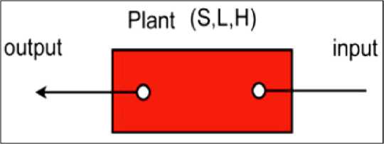
Figure 12. Input-Output device with system parameterized by (S, L, H)

The dynamics of a system coupled to input fields is given by the quantum Langevin equations.

As mentioned above, we describe each unit by a tuple

G = ( S,L, H ) (23)

where H is the internal Hamiltonian of the system; S is a n × n unitary matrix with operator entries and is called a scattering matrix; L = ( L,..., L_n ) T is a vector of operators through which the system couples to the inputs, with one for each input. We denote the inputs to the system by b_in ( t ) = [ b_x ( t ),..., b_n ( t ) ] in which each of the b ( t ) , ( i = 1,..., n ) , are separate input fields, all initially in the vacuum state. The notation given in Eq. (23) can be used to describe a wide range of dynamical and static systems. A single quantum input-output system can be written as G _Bs= ( I ,L, H ) , and a quantum beam splitter is given by G bs = ( S,0,0 ) .

Remark . Each input-output component in a photonic circuit is described by a triple ( S , L, H ) , where S is the scattering matrix of the component, L is the coupling vector of the component, and H is the Hamiltonian of the component’s internal degrees of freedom. S is required to be a unitary matrix, and its matrix elements can in general be operators on the Hilbert space of the component’s internal degrees of freedom (although they are usually just complex numbers). The elements of L can also be operators, in which case they describe the way that external fields couple to the component’s internal degrees of freedom. H plays the usual role of determining the (autonomous) time evolution of the component’s internal degrees of freedom. The dimension of L is equal to the number of input-output ports n that the component has (every port must be both an input and an output); the dimension of S is n x n ; the Hamiltonian H is scalar (see, Fig. 13).

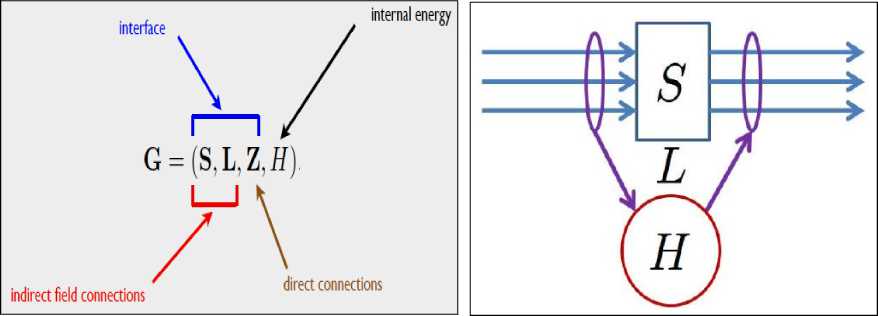
Figure 13. ( S,L, H ) -model

We now present the Langevin equations describing input-output systems in more generality. To begin, we introduce a vector of quantum Wiener processes B ( t ) and a matrix of quantum Poisson process Л ( t ) as

( B 1 )

( b.

B„ ^

^{B (} t )=; , ^{Л (} t ) =

V Bn 7

в

V ^n 1

B J nn

These noise processes are integrals of the input fields:

Bi(t) = JЛ T dT,  Bj (t) = i0ТЬ^(Т) bj (T) dT .                     (25)

The increments of these gauge processes B ( t ), Л ( t ) satisfy the quantum stochastic calculus relations given in Table 2.

Table 2: Quantum Ito Rule for quantum stochastic calculus

dXjdY	dB	dX	(/Bt	dt
d^	0	dB	dt	0
dX	0	dX	dB^	0
dB	0	0	0	0
dt	0	0	0	0

Let V (t) be the unitary evolution operator of the total system composed of the controlled system and the input field, then the evolution equation of the total system can be written as dV (t ) = ^Tr [( S -1) d ЛT ] + dBt L - LjS dB -- Lj Ldt - iHdt j V (t)

with initial condition V ( 0 ) = I .

In the Heisenberg picture, the system operator X (t) = V (t) XV ’ ( t ) satisfies the following quantum stochastic differential equation

dX(t) = {ll(,)[X(t)]-i[X(t),H (t)]} dt + dB (t)S’ (t)[X (t),L(t)] + [L’ (t), X (t)] S (t) dB (t) + Tr {[St (t) X (t) S (t)-X (t)] dЛT (t)}, where the Liouville superoperator Lq^ (•) is defined by

n

L I ( X ) = T^L ’ [ X ,L ] +-[ L ’ , X ] ^L =^- j X , L j ]+-[ L j , X ] L j ,         (28)

2              2              j = 1 1 2               2

which is of the standard Lindblad form. Similar, the output fields corresponding to the inputs B(t) and Poisson process Л( t) are given by B (t) = V’ (t) B (t) V (t), Лои1 (t) = V’ (t) Л (t) V (t) , from which we obtain the following input-output relation dBout (t) = S (t) dB (t) + L (t) dt,

dЛ_ош ( t ) = S * ( t ) d Л ( t ) S T ( t ) + S * ( t ) dB* ( t ) L^T ( t ) + L * ( t ) d B^T ( t ) S T ( t ) + L * ( t ) L T ( t ) dt

It can be verified that the increments dB_0llf, dЛ_оиt , of the output processes also satisfy the rules of quantum stochastic calculus shown in Table 1.

For linear quantum systems, the quantum Langevin equations can be solved directly. In order to perform calculations for nonlinear quantum systems, one must transform the Heisenberg equations of the input-output formalism to master equations. The corresponding master equations are p = -i [H, p] + ^ [ LjPLj' -1 LjLP -1 PLjLj V       2        2

Although the scattering matrix S does not appear in the master equation (8), it affects the input-output relation of the system as shown in Eq. (7) and thus will affect the dynamics of more complex quantum inputoutput systems, such as the quantum cascade systems which will be specified below.

To connect the outputs of one unit to the inputs of another, so as to form an arbitrary network, we need only two rules. The first is merely a rule that says how to represent a universe that contains more than one separate unit, none of which are connected. If we have the two units G₁ = ( SpLp H ) and G₂ = (S₂ , L₂ , H ) , the unit that describes both these units with no connections between them is

G i ( G 2

0 S 2

L2

Gough and James refer to this rule as the concatenation product .

The second rule for combing circuit elements tells us how to determine the unit that describes a network in which the outputs of a unit G are connected to the inputs of a unit G . This rule is

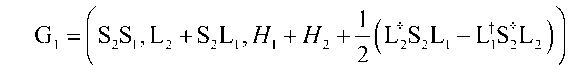
and is called the series product . The concatenation and series products can also be used to decompose a given system into subsystems, and are thus fundamental to feedforward and feedback control.

Quantum transfer function model

The Collet-Gardiner/Hudson-Parthasarathy cascade connections can be used to model essentially any network. However, for linear systems, time-delays and quantum amplifiers can be modeled more easily in frequency space. If we specialize the network formalism of Gough and James so that all the systems are linear, and transform the equations of motion to frequency space, then we have the method of quantum transfer functions.

A general linear quantum network described by the tuple ( S , L , H ) satisfies the following conditions : (i) the entries of the scattering matrix S are scalars; (ii) the dissipation operators L are linear combinations of the a and a ^† ; and (iii) the system Hamiltonian H is a quadratic function of the a and a ^† . To elucidate the transfer function method further, we consider a useful special case, in which each system is a harmonic oscillator, and the field coupling operators are linear combinations of only the annihilation operators. In this case, the Langevin equations for the annihilation operators are not coupled to those for the creation operators. The annihilation operators for the n oscillators, { a : j = 1,..., n } , satisfy the commutation relations

[ aj, a ^ J = ^ , [ aj, a_k J = |^ a _y", a ^ J = 0 . The total Hamiltonian is H = ^ ^ ^ a J a _y and the coupling operators Lj = ^ . _kc_jka_k , and so we can simplify the SLH formalism, writing the tuple

Where

C

( ^

Q

I ^to r

co J nn

If we now introduce an operator vector, which we will call the state vector of the system, a = ( a_x,...,a_n ) ^T , then from Eqs. (5) and (7), we can obtain the following Langevin equation and inputoutput relation:

a (t ) = Aa (t) —C 'Sb,, (t),  b _ = Sb,, (t) + Ca (t), where A = —C'C /2 — iQ.

We can now transform these equations to frequency space by taking either the Laplace transform or the Fourier transform. Using the Fourier transform, defined as

R (V) = JO exp (—Vt)R (t) dt,(35)

the Langevin equations can be rearranged to obtain a (V) = —( VIn — A)-1 C 'Sbin (V) ,  b out (V)= Sb, (V) + Ca (V)

From Eqs. (14), we can obtain the input-output relation of the whole system or network b out (V) = E( V) b in (V)

where E ( V ) is the transfer function of the linear quantum system which can be calculated by

E(v) = S — C ( VIn — A )-1 C 'S

The input-output relation (15) show the linear map between the input and output of the linear quantum system given by Eqs. (12).

The quantum transfer function approach is useful for a number of reasons. While the time-domain network formalism can describe essentially any network, it cannot be used to incorporate static models of nonconservative elements, such as quantum amplifiers, and such components must be treated as dynamical systems. In frequency space, a static model of a quantum amplifier is simply a Bogoliubov transformation. Time delays are also much simpler to include in frequency space, and of course frequency space has the advantage that the transfer function of two cascaded systems is merely the product of the transfer functions of each.

Quantum filters: Physical motivation

As above mentioned the theory of quantum filtering was developed by V. P. Belavkin [11], and represents the continuation of the work of Kalman, Stratonovich, Kushner, Zakai, etc.

To better understand quantum filtering, let us consider an indirect quantum measurement, which is achieved by interacting the measured system with a bath via a system operator L , and then making a measurement on the bath. The bath is a continuum of harmonic oscillators of different frequencies. The bath also describes a field, such as the electromagnetic field, in which the oscillators are the modes of the field. The Hamiltonian of the total system composed of the measured system and the bath is given by

H = H + Hb + Hint, Hb =J dtotob' (^)b(^), Hmt= iJ dm[k(^)b' (^)L — hc] , where Hs is the free Hamiltonian of the measured system, b'(m) and b (m) are the creation and annihilation operators of the bath mode with frequency m , and satisfy I b (m), b'(m) I = 5(m — m). The bath mode with frequency to interacts with the system via the system operator L, where k(to) is the corresponding coupling strength. Hereafter we set = 11. The total Hamiltonian H can be re-expressed in the interaction picture as

H_{ef f} = exp ( iH_bt )( H + H _int) exp ( - iH_bt ) = H_s + i J d to [ k( to )e^iOtb ¹ ( to )L — hc ] .

We now introduce the Markovian assumption

k ' '^21

which allows the Hamiltonian H to be

expressed as H

= Hs + i V/ [b'in (t) L — Lbin (t )] , where bin ( 4) = ^= J , dtoe"^b (to)

is the Fourier

transform of the bath modes. The operator b_in ( t ) is, in fact, the time-varying field that is incident on, and thus the input to, the system, and satisfies ^ b_in ( t ) , b\_n ( t ) ^ = 5 ( t — t ) . We now define a new bath operator

Bin (t) = Jtb, (T)dT, which is called a quantum Wiener process. If we assume that the bath is initially in a vacuum state, the increment of the quantum Wiener process dB and its conjugate dB† satisfy the following algebraic conditions: dBindB\n = dt, dB\.ndBin = dBVndB\n = dBindBin = 0 . These are the quantum version of Ito rule. With the above notation, in the Heisenberg picture, an arbitrary system operator X (t) satisfies the following quantum stochastic differential equation dX = — i [X, Hs ] dt + Y {L [X, L] + [L, X] l} dt + 77 {dBin [L, X] + [X, L] dB1 in} .     (39)

It is then possible to define an output filed bout (t) which describes the field leaving the system after it has interacted with it, and we can similarly define its Ito increment Bout (t) = J.bout (r)dr . The celebrated input-output relation for the system can then be written as dB„ = dB, + YLL ■

If homodyne detection is performed on the output field Bout (t), then the operator corresponding to the measured output is dYout = —^( dBout + dB\Mt), and satisfies the following equation ou ^V OU OU 7

dY- =( L + L) dt

⁺ ^ ( dB , + dB ''' in ) .

With the above preparation, we can now present the main results of quantum filtering theory . The purpose of quantum filtering is to provide an estimate п ( X ) of the value of the system observable X , at time t , given the stream of measurement results up until that time. We will define this estimate as the expectation value of X given the measurement results.

To obtain п ( X ) we first define Y_Mt = { X : = f ( Y_out) , f : R ^ C } , which is the smallest commutative algebra generated by the observation process Y , and denote P as the probability measure on Y . The estimate п ( X ) is then the conditional expectation of X on Y_Mt :

п ( X ) = P ( X Y out ) .                                  (40)

From the definition of п ( X ) given in Eq. (40), it can be proved that we can obtain the following dynamical equation for п ( X ) and the corresponding output equation from dX and dB_out as following:

^dY out = ^п ( ^{L +} L )

dп (X) = п [L (X)] dt + Jy [п (LX + XL)-п (L + L) п (X)] dW dt + -1= dW, V Y

where L ( X ) is the Liouville superoperator of the system defined as

L ( X ) = - i [ X, H_s ] + у ^ L XL - 1 L LX + 1 XL L

The process W (t) in Eqs. (41) is called the innovation process of quantum filtering, and has been shown to be a classical Wiener process. The increment of W (t) satisfies the following classical Ito relations E (dW) = 0,  (dW)2 = dt, where E (·) is the ensemble of the stochastic process induced by dW. The dynamical equation (41) of п (X) is called the quantum filtering equation. The filtering equation (41) and the output equation (41) are the main results of quantum filtering theory.

Additionally, we can convert the filtering equation (41) from the Heisenberg picture to the Schrödinger picture, and thus obtain a stochastic equation for the evolution of the density matrix. To show this, we use the fact that the density operator p satisfies Tr [п ( X ) p ] = Tr ( X_o p ) , where p is the initial density operator of the system and X is the corresponding system observable in the Schrödinger picture. Substituting Eq. (41) into the above relation, the system density operator p evolves according to the following stochastic master equation :

• dpc = — i [Hs , pc ] dt + 1 ( 2LpcL — LLpc — pcLL ) dt + { Lpc + pcL — Tr [( L + L ) pc ]} dW (42)

From Eq. (1), we have p = P ( p Y_{ou z}) . That is, p is the conditional expectation of the density operator p which is defined by Tr [ X p ] = Tr ( X_o p ) . The stochastic master equation (42) is also often referred to as quantum filtering equation .

Thus, the quantum stochastic differential equation (40) and the output equation (41) give the dynamics of the operators that describe the measured quantum system. These equations are driven by the quantum Wiener noise dB , and are thus defined on a quantum probability space. As a comparison, the quantum filtering equation (41) (or the stochastic master equation (42)) and the output equation (41) give the observers state-of-knowledge of the measured quantum system based on the information extracted by the quantum measurement. These equations are driven by the classical Wiener noise dW and thus defined on a classical probability space. Therefore in quantum filtering theory we use a classical stochastic system to mimic the dynamics of a quantum stochastic model, which is why we refer to quantum filtering as a bridge between a quantum probability model and a classical probability model.

Example . Partial information about state of high Q cavity modes is obtained by measuring Rydberg atoms that passed one-to-one through the cavity (see Figure 14).

Qubits (Rydberg atoms) are passed through a cavity one by one. At any one time there will be at most one qubit inside the cavity, and we measure the outgoing qubits one-by-one. The measurement bit y is sent into a filter which estimates the state of the cavity mode, and then an instruction is sent to the actuator so as to control the mode. The measurement results can be used to apply a feedback action on the cavity mode.

We consider a quantum mechanical system which is probed by a two-level atom (qubit).

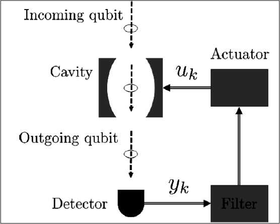
Figure 14. A schematic of the LKB photon experiment

The qubit is in input state Ф) initially. The unitary interaction between the cavity mode and the probe qubit leads to a change of state in the Schrödinger picture:

। ^ ®h)=и i^ ®h)

We take the interaction time т to be very small and assume that the unitary has the form

U = exp {V L L ® a*

—

LLL ® a — irH ® I2 }D 1 + TLL ® a

• — LLL®a — т| -L*L + iH |® /2 + •••

1 2            )    ²

We now measure the spin a_x of the qubit and record the eigenvalues 7 7 = ± 1 corresponding to eigen-

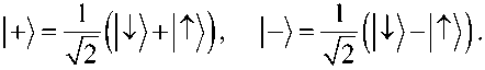
± 1 are

p ± = ^- ± ^{- L}^^{LL +} L 1 ^ +'"

After measurement, the system state becomes (up to normalization)

I^7) ^k)+^LLVn—тI -LL+iH 11^)+

This is interpreted as a discrete-time quantum Kalman filter [27].

For a continuous time limit we have (due to a central limit effect) т h^ dt, Tn h^ dY (t), where Y (t) , the continuous time measurement readout, will be diffusion process. The limit equation is d\%h = L Xt)dYt-f1LL +iH j|%t}dI (t),

and we refer to this as the Belavkin-Zakai equation as it plays the same role as the Zakai equation in Belavkin’s theory of quantum filtering. In general | / J is not normalized, but it is easy to obtain the equation for the normalized state ^ J = | x ) /1|| X )||, we find the Stochastic Schrodinger equation

d kt) =iH Wd -1 ( L - ^t )* (L - ^t )| V?)dt + (L - ^t) ^dl (t),

where \ □ ^ |L + L k )’ d (t )□ dY - fyd •

Mathematically I ( t ) has the statistics of a Wiener process, and its increment di ( t ) is the difference between what we observe, dY ( t ) , and what we would expect to get ^ |L + L | k ) • It is convenient to frame this in the Heisenberg picture.

Information-theoretical bounds and physical limits on quantum control

We discuss an information-theoretic framework for analyzing control systems based on the close relationship of controllers to communication channels. A communication channel takes an input state and transforms it into an output state. A controller, similarly, takes the initial state of a system, to be controlled and transforms it into a target state. In thus sense, a controller can be thought of as an actuation channel that acts on inputs to produce desired outputs. In this transformation process, two different control strategies can be adopted: (i) the controlled (open-loop control); or (ii) the controller enacts an actuation dynamics that is based on some information about the state of the controlled system (closed-loop control). Using this communication channel model of control, we provide necessary and sufficient conditions for a system to be perfectly controllable and perfectly observable in terms of information and entropy [31-38].

New derivations of the advantage afforded by closed-loop control and proposing an information-based optimality criterion for control systems are described. In addition, we discuss a quantitative trade-off between the amount of information gathered by a closed-loop controller and its relative performance advantage over an open-loop controller in stabilizing a system.

Information control system theory: Introduction

It is common in studying controllers to describe the interplay between the sensors used to estimate the state of a system, intended to be controlled, and the actuators used to actually modify the dynamics of the controlled system, as a transfer of information involving three steps: estimation, decision, and actuation. In the first step sensors are used to gather information from the controlled system in the form of data relative to its state (estimation step). This information is then processed according to some plan or control strategy in order to determine which control dynamics is to be applied (decision step), to be finally transferred to the actuators which feed the processed information back to the controlled system to modify its dynamics, typically with the goal to decreasing the uncertainty in the value of the system’s variables (actuation step).

Whether or not the estimation step is present in this sequence is optional, and determines which type of control strategy is used. In so-called closed-loop or feedback control techniques, actuators rely explicitly on the information provided by sensors to apply the actuation dynamics, whereas in open-loop control there is no estimation step preceding the actuation step. In other words, an open-loop controller distinguishes itself from a closed-loop controller in that it does not need a continual input of ‘selective’ information to work: like a throttle or a hand brake, it implements a control action independently of the state of the controlled system. In this respect, open-loop control techniques represent a subclass of closed-loop controls that neglect the information made available by estimation.

Since control is fundamentally about information (getting it, processing it, and applying it), it is perhaps surprising to note that few efforts have been made to develop a quantitative theory of controllers focused on a clear and rigorous definition of information. Indeed, although controllers have been described by numerous authors as information gathering and using systems, and despite many results related to this problem, there exists at present no general information-theoretic formalism characterizing the exchange of information between a controlled system and a controller, and more importantly, which allows for the assignation of a definite value of information in control processes. To address this deficiency, we present in this section with a quantitative study of the role of information in control. The basis of the results was first elaborated in [34], and draws upon the work of several of the papers cited above by bringing together some aspects of dynamical systems, information theory, in addition to probabilistic networks to construct control models in the context of which quantities analogous to entropy can be defined.

Central to this approach is the notion of a communication channel, and its extension to the idea of control channels. As originally proposed by Shannon, a (memoryless) communication channel can be represented mathematically by a probability transition matrix, say p ( ^|x ) , relating the two random variables X and Y which are interpreted, respectively, as the input and the output of the channel. We adapt this common probabilistic picture of communication engineering to describe the operation of a basic control setup, composed of a sensor linked to an actuator, in terms of two channels: one coupling the initial state of the system to be controlled and the state of the sensor (sensor channel), and another one describing the state evolution of the controlled system as influenced by the sensor-actuator’s states (actuation channel).

We use this model in conjunction with the properties of entropy-like quantities to exhibit fundamental results pertaining to control systems. As a first of these results, we show that the classical definition of controllability, a concept well-known to the field of control theory, can be rephrased in an information-theoretic fashion. This definition is used, in turn, to show that a system is perfectly controllable upon the application of controls if, and only if, the target state of that system is statistically independent of any other external systems playing the role of noise sources. A similar information-theoretic result is also derived for the complementary concept of observability. Moreover, we provide bounds on the amount of information a feedback controller must gather in order to stabilize the state of a system.

More precisely, we prove that the amount of information gathered by the controller must be bounded below by the difference: AH_c[osed -AH maX_n , where A H_closed is the closed-loop entropy reduction that results from utilizing information in the control process, and A H maX_n is the maximum decrease of entropy attainable when restricted to open-loop control techniques. This last result, as we will see, can be used to define an information-based optimally criterion for control systems.

Remark. The idea of reducing the entropy a system using information gather from estimating its state is not novel by itself. Indeed, as he wondered about the validity of the second law if thermodynamics, the physicist James Clerk Maxwell was probably the first to imagine in 1897 a device (or a ‘demon’ as it was later called) whose task is to reduce the entropy of a gas using information about the positions and velocities of the particles forming the gas. In the more specific context of control theory, the problem of reducing the entropy of a dynamical system has also been investigates notably by Poplavskii and by Weidmann. Pop-lavckii analyzed the information gathered by sensors in terms of Brillouin’s notion of negentropy, and derived a series of physical limits to control. His study focuses on the sensor part of controllers, leaving aside the actuation process which, as will be shown, can be also treated in an information-theoretic fashion. In a similar way, Weidmann performed an information-based analysis of a class of linear controllers having measure preserving sensors.

We build on these studies and go further by presenting results which apply equally to linear and nonlinear systems, and can be generalized with the aid of a few modifications to encompass continuous-space systems as well as continuous-time dynamics. To illustrate this scope of applications, we study specific examples of control systems. Among these, we consider two variants of proportional controllers, which play a predominant role in the design to present-day controllers, on addition to complete our numerical investigation of noise-perturbed chaotic controllers. In addition, we discuss a quantitative trade-off between the amount of information gathered by a closed-loop controller and its relative performance advantage over an open-loop controller in stabilizing a system. Finally, we remark on the relationship of frameworks with thermodynamics and optimal control theory [35, 36].

Control and thermodynamics

The reader familiar with thermodynamics may have note a strong similarly between the functioning of a controller, when viewed as a device aimed at reducing the entropy of a system, and the thought experiment of Maxwell known a the Maxwell’s demon paradox. Such a similarly was already noted in the Introduction section of this work. In the case of Maxwell’s demon, the system to be controlled or ‘cooled’ is a volume of gas; the entropy to be reduced is the equilibrium thermodynamic entropy of the gas; and the ‘pieces’ of information gathered by the controller (the demon) are the velocities of the atoms or molecules constituting the gas. When applied to this scheme, our result on closed-loop optimality can be translated into an absolute limit to the ability of the demon, or any control devices, to convert heat to work. Indeed, consider a feedback controller operating in a cyclic fashion on a system in contact with a heat reservoir at temperature T. According to Clausius law of thermodynamic, the amount of heat AQclosed extracted by the controller upon reducing the entropy of the controlled system by a concomitant amount AHdosed must be such that

A Q, = =kkT ln2 ) A H,                   (45)

closed       B               closed

In the above equation, k is the Boltzmann constant which provides the necessary conversion between units of energy (Joule) and units if temperature (Kelvin); the constant ln 2 arises because physicists usually prefer to express logarithms in base e . From the closed-loop optimality theorem, we then write

AQ ciosed ^ ( kT ln2 ) [A H „ mX + 1 ( X ; C ) ]=A Q" + ( к в Т ln2 ) I ( X ; C ) ,          (46)

where A Q™_n = ( k_BT ln2 ) A H mX . This limit should be compared with analogous results found by other authors on the subject of thermodynamics demons.

It should be remarked that the connection between the problem of Maxwell’s demon, thermodynamics, and control is effective only to the extent that Clausius law provides a link between entropy and the physically measurable quantity that is energy. But, of course, the notion of entropy is a more general notion than what is implied by Clausius law; it can be defined in relation to several situation which have no direct relationship whatsoever with physics (e.g., coding theory, rate distortion theory, decision theory). This versatility of entropy is implicit here. Our results do not rely on thermodynamic principles, or even physical principles for that matter, to be true. They constitute valid results derived in the context of a general model of control processes whose precise nature is yet to be specified.

Entropy and optimal control theory

Consideration of entropy as a measure of dispersion and uncertainty led us to choose this quantity as a control function of interest, but other information0theorretic quantities may well have been chosen instead if different control applications require so. From the point of view of optimal control theory, all that is required is to minimize a desired performance criterion (a cost or a Lyapunov function), such as the distance to a target point or the energy consumption, while achieving some desired dynamic performance stability) using a set of permissible controls. For example, one may be interested in maximizing AHclosed instead of minimizing this quantity if destabilization (anti-control) mixing is an issue. As other examples, let us mention the minimization of the relative entropy distance between the distribution of the state of a controlled system and some target distribution, the problem of coding, as well as the minimization of rate-like functions on decision or game theory.

The purpose of quantum control in general case is defined as intelligent process of a reduction of the entropy of the control system Q , e.g., quantum Maxwell demon, quantum bang-bang control, and quantum error correction code. Fundamental limits on the controllability of quantum mechanical system can be discussed in the light of quantum information theory: The amount of entropy reduction that can be extracted from a quantum system by feedback controller is upper bounded by a sum of the decrease of entropy achievable in open-loop control and the mutual information between the quantum system and the controller. This upper bound sets a fundamental limit on the performance of any quantum controllers whose designs are based on the possibilities to attain low entropy states. An application of this approach pertaining to quantum error correction is also discussed.

Remark . The rapid development of quantum information technology suggests that quantum control theory might profitably be reexamined from the perspective of quantum information theory. In this section we address explicitly the role of quantum information and entropy in quantum control processes. Specifically, based on classical theories, we prove several limiting results relating to the ability of a control device to reduce the von Neumann entropy S = Tr ( p Q log p Q ) of an arbitrary quantum system p Q in the cases where (i) a controller independently acts to the state of the system (open-loop control) and (ii) the control action is influenced by some information gathered from the system (feedback control).

When a quantum system Q initially prepared in a pure state p interacts with an environment represented by the density operator p(En), the system Q and environment evolve according to the joint unitary evolution operator U . Then the density operator for the system Q and environment is p = UqeДp ® P(En)) U1 qe„• After performing a partial trace over environment variables, the marginal density matrix of the system Q is represented by a completely positive and trace preserving map E , which takes the form pQ = E (p ) = Z E,pE1 , where the Kraus operators Ef ’s satisfy the trace preserving properi ty, i.e., Z E1E = I. This equation is known as operator-valued representation of the quantum operation E .

i

Unitary evolution of the quantum system is a special case in which there is only one non-zero term in the operator sum; if there are two or more terms, the pure initial state becomes a mixed state. Therefore, the von Neumann entropy of the system Q increases, i.e., A ( Q ) = A ( p Q ) >  S ( p ) , because of the interaction with environment. In this case the purpose of quantum control is defined as a reduction of the entropy of the system Q . We will consider the fundamental limits on the control of quantum mechanical systems from the viewpoint of quantum information inequalities.

Information-theoretic analysis of open-loop and closed-loop (feedback) quantum control systems

We address explicitly the role of quantum information and entropy in quantum control process of a QA-evolution. Specifically, we consider several limiting results, based on classical theories, relating to the ability of a control object to reduce the von Neumann entropy S = Tr (pQ logpQ ) of an arbitrary system pQ in the cases where (i) controller independently acts to the state of the system (open-loop control); and (ii) the control action is influenced by some information gathered from the system (feedback control). The infor- mation-theoretic analysis of open-loop and closed-loop (feedback) control gives the fundamental limits on the control of quantum mechanical system as QA from the viewpoint of quantum information theory [37-42].

• A . Quantum open-loop control . We will consider a joint unitary evolution (a control unitary operation) of quantum system Q and controller C . Let the quantum system Q and the controller C be disentangled before the control unitary operation. We also assume that the state of system Q and C are respectively given by p Q = E ( p ₀ ) = Z Ep^E i and p = Z P j i K i l. Here i is an orthonormal basis of system C

i                             iC                  C and Z p4 = 1. Therefore, the state of the joint system (QC) is given by: i

P^ ^Q = p ^Q ® p ^C = Z p p j I Cc ^ I, p ^Q = E p E .

• i ,

In order to reduce the entropy of the system Q , a control unitary transformation U is applied to joint system ( QC ) . Then the system ( QC ) undergoes the evolution:

QC         QC † p          opp     op

We shall consider two types of control unitary operation: (i) global unitary operation; and (ii) local quantum operation and classical communication (LOCC).

Figures 15 a,b shown these types of control [37, 38].

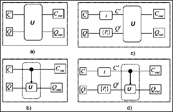
Figure 15: Quantum Control Schemes

Remark . In Figure 15 (a) quantum open-loop control using global unitary transformations; (b) quantum open-loop control using LOCC; (c) quantum feedback control using global unitary transformations; (d) quantum feedback control using LOCC

A1 . Global unitary operation . In former case, the entropy of the total system becomes: S ( Q, C ) = S ( Q out , C out ) <  S ( Q out ) + S ( C out ) , where we have used the subaddivity of the entropy.

From this inequality, we finally obtain the entropy reduction A S op^{e n} as:

A SQ>™ = S (Q)- S (Qout )< S ( Cout) — S ( C ),

with the equality iff: p QC ou = p ^Q ® p^c C ou .

Therefore, the entropy reduction is upper bounded by the maximum amount of the entropy increase of the controller C .

A2. LOCC-operation . In the case of LOCC-strategy the control unitary operation is given by U op = E U ® I Oc ( ^z ' I. Therefore, the state after the open-loop control becomes

i

P ' ' = U p = £ pU j, |z)c ( i |.

• i ,    j

Then, the marginal density operator of Q is given by:

p ^Q _ Tr_c ( p >■^{, c ,} ) = £ рД р- ' Ц ^f .

i

Now using the concavity of the von Neumann entropy as

⁵ f z PiPi

V i       )

< E Pi^{s (} P i) , we see that:

• 5 ( e _ ) = ' E pu, P ’ u;  E p5 ( u р и , ) = 5 ( q ) .

  
  

V i                  ) i

Therefore for open-loop control the LOCC-strategy finally: A 5Cp^en <  0 . This means that we can never reduce the entropy of system Q in contrast with the case of the global unitary operation strategy.

• B .    Quantum feedback control . In this case, the controller C performs measurements on the system Q and feeds back the results of these measurements by applying operations that are the functions of the measurement results. Although both the system Q and the controller C are quantum mechanical in principle, the feedback operations we consider here involve feeding back classical information. To analyze quantum feedback control, we need to consider quantum measurement processes. We consider (for simplicity) a POVM measurement in which the entropy of the system Q does not decrease, e.g., the conventional von Neumann measurement model.

As in the case of open-loop control, we shall investigate two types of control strategies (see Figures 15 c,d).

• B1 .    Global unitary operation . Figure 15 c shows a basic quantum feedback control using a global control unitary operation. The entropy of the controller C is calculated as

s ( c„. ) = s ( Q„ , C„ ) - 5 ( Q ,, ) + 1 ( Q ,, : C_, )

= 5 ( Q ‘ , C ' ) - S ( Q ,, ) + 1 ( Q ,, : C ,, )                                    (49)

<  5(Q)-5(Q,, >  + 5(C') +1 (Q,, : C,„)-1 (Q': C')

En ropy defec of con rol objec                          Mu ual informa ion loss

Here I ( A : B ) = 5 ( A ) + 5 ( B ) — 5 ( A, B ) is the quantum mutual information of systems A and B .

Therefore, the entropy reduction for quantum feedback using the global unitary operation is given by the following:

A '      = S ( Q ) - S ( Q „) <  S ( Q',C ' ) - S ( Q. ) + 1 ( Q„„ : C. )

= S ( C . .) - S ( C ' ) + 1 ( Q' : C ' ) - 1 ( Q..- C... )                         (50)

Entropy defect of controller            Mutual information loss

< max A S O”™ + 1 (Q' : C ' )

Here max A SOpe" is the maximum entropy reduction attained by restricting the control model to open-UQ loop system.

The equality holds iff p ^Q = p ^Q and

S ( C .) - S ( C ' ) - 1 ( Q,„ : C „„ ) = max A SO” .                     (51)

Therefore, the maximum improvement that closed loop can give over open-loop control is limited by the quantum mutual information obtained by the controller C .

Now we shall consider quantum feedback control using the LOCC.

• B2.    LOCC-operation . Figure15 d show the quantum feedback control scheme using the LOCC. In this case the entropy reduction is upper bounded by the quantum mutual information between intermediate quantum states Q ' of control object and controller C ' , i.e.,

A S Feedback <  I ( Q ‘ : C ' ) .                                         (52)

ii

From the inequality of the entropy exchange S_ex ( p , E ) for a quantum operation as

S ( E ( p ) ) - S ( p ) + S ex ( p , E ) S 0

it follow that

S ( e . ,) - S ( Q ) + S„ ( p ^Q , C ) s 0 .

Thus we inequality for the entropy reduction,

A S Q™ = S ( Q ) - S ( Q ou, ) < S „ ( p ^Q , C ) .                     (53)

The entropy exchange is not greater than the Shannon entropy for the probabilities

P i = Tr ( UP p Q P'U ' ) .

Thus, S „ ( p ^Q , C ) <  H ( p_z^q ) , where equality holds iff the operator UP is a canonical decomposition of C respect to p ^Q . Therefore we have:

A S QF — <  H ( p , ) = _ ^ p , _]og p, .                       (54)

i

Remark . The joint state after measurement is given by

Р°C ' = Z PiP°Pi ^{f 0} V)c (i l = Z PqPi ⁰1 i)c (i I, ii

P PQP" where p. = —----—. Therefore the entropy of the system (Q C ) is given by piq

S (Q , C ■) = S f^ p’p,0 Vc.il 0 = H (P ) + Z P1S (P.) = H (Pl)           (55)V                  / where in the second equality the joint entropy theorem is used. The marginal density operators of subsystems Q ’ and C ‘  are respectively given by p^ =ZP^WA and PC'=ZPiqli i so we have:

ii

S ( q -)= S (c ■)=H (pq).

Therefore the mutual information between subsystems Q ’ and C ‘ is

I ( Q' : C ‘ ) = S ( Q ‘ ) + S ( C ‘ ) - S ( Q\C ‘ ) = H ( p q ) .                    (56)

While in the case of the quantum feedback using LOCC, H ( p i ) = I ( Q’ : C ‘ ) , the entropy reduction is given by

Д S^FF^e(Z^^k <  I ( Q’ : C ') = H ( pq ) .                              (57)

This implies that the maximum amount of entropy reduction is exactly equal to the maximum mutual information between subsystems Q’ and C^f , i.e., I ( Q ‘ : C ') .

Remark . The quantum mutual information I ( A : B ) is related to the correlation between subsystems A and B : If joint system A and B is a product state, then I ( A : B ) = 0 ; however, I ( A : B ) > 0 if the subsystems A and B are (classically or quantum mechanically) correlated. In the case of the quantum feedback (see, Figures 15 c,d) the quantum measurement germinates not quantum but classical correlation [42] between Q and C .

Therefore, we can conclude that the classical correlation between Q ‘ and C ‘ can increase the amount the entropy reduction in compared with the case of the quantum open-loop control.

These results are the background for information analysis of successful solution searching from QAs evolution.

We give an introduction to the topic of Quantum Feedback Control , explaining what its objectives are, and describing some of its physical resources, limitations and information bounds. Reader that not familiar with classical feedback and stochastic control can find the necessary information in Appendices.

Conclusions

In present article we are concentrate our attention on the description of efficient quantum feedback control models, its physical limits and information bounds and tradeoffs between performance , stability and robustness . We are considered separating the problem of designing Hamiltonian quantum feedback control algorithm into a measurement (estimation) strategy and a feedback (control) strategy, and we consider optimizing desirable properties of each under the minimal constraint that the available strength of both is limited.

These motivate concepts of information extraction and disturbance that are distinct from those usually considered in quantum information theory. Mathematical background is described in [39-42].

We are focuses on the design of control fields that achieve given state transfers with the minimum amount of energy expenditure. Besides their inherent mathematical interest, such optimal designs are closely tied to the dynamics of the underlying system and reveal much about the interplay of dynamics and control. We consider energy-optimal transfers in a general isolated quantum system, for example an atom or a molecule. By examining the large-time limit of these optimal transfer problems, we uncover the general structure of the optimal controls. Moreover, we reduce the computational complexity of the problem significantly.

While feedback control of the system Hamiltonian is sufficient to cover the full classical control problem, it is not sufficient in the quantum case. This is because, in general, the quantum measurement process disturbs and changes the dynamics of the system. Consequently the formulation of the full quantum feedback control problem must also allow for the possibility that the measurement process is also changed as a result of the observations.

We examine similar problems for open quantum systems, that is, quantum systems that interact with their environment. This interaction creates dissipative effects in the system. Although one usually wants to resist these effects, there are instances, such as the cooling of internal molecular motion, that one can effectively use dissipation mechanisms to one’s advantage. We apply techniques similar to those developed for isolated systems to design “cooling” electric (laser) fields for molecular rotations. We will look at the formulation of quantum feedback control theory for continuously observed open quantum systems in a manner that highlights both the similarities and differences between classical and quantum control theory. We will involve a discussion of special topics in the field and is meant to provide a casual overview of current experiments in quantum control.

This review was assembled from various lecture notes, (conference and meeting) presentations and research papers of many authors, and so we apologize for the inevitable inconsistencies that resulted. Neils Bohr says: “ Never speak more than you think .” In References we are introduced the employment original publications according to Neils Bohr recommendation.

Appendix 1. Boson and Fermion Fields

We may think of observables as quantum random variables , and the key distinction with classical probability is that quantum random variables do not in general commute. Indeed, if ( Q , F , P ) is a classical probability space then classical bounded real-valued random variables in L ( Q , F , P ) have an interpretation as multiplication operators that map the Hilbert space L ( Q , F , P ) to itself. Since all such operators commute with one another, bounded classical real-valued random variables are thus isomorphic to (and can be viewed as) commuting observables on L ( Q , F , P ) .

In quantum field theory, a one dimensional quantum field (with parameter t ) consists of a collection of systems each with annihilation a ( t ) and creation operators a * ( t ) used to describe the annihilation and creation of quanta or particles at index location or point t . a ( t ) and a * ( t ) are referred to as field operators, the annihilation and creation field operators, respectively. The index t may represent a range of variables, including position, frequency and time, and we assume here that t lies in a continuous interval T in . Basic considerations lead to the postulate that the annihilation and creation operators must satisfy either the commutation relations

[ a ( t ) , a * ( t ') ^| = 5 ( t - t ') (A1.1) or the anticommutation relations

{ a (1), a *( 1')} = 5 (1 -1')                                      (A1.2)

for all 1 , 1 'g T , where 5 ( 1 ) denotes the Dirac delta distribution.

Fields that satisfy the commutation relations (A1.1) are called boson fields (e.g. photons), while fields that satisfy the anticommutation relations (A1.2) are called fermion fields (e.g. electrons). We will take the parameter t to be time and T = [ 0, да ) . In this case a ( 1 ) has the interpretation of annihilation of a photon

(in the case of a bosonic field) or electron (in the case of fermionic field) at time t , whereas a * ( 1 ) has the interpretation of creation a photon (in the case of bosons) or electron (in the case of fermions) at time t. One can imagine these fields as a continuous collection or stream of distinct quantum systems (one quantum system for each t ) hence, informally, quantum fields can be defined on some continuous tensor product

Hilbert space H = ®Zep ^H, where H is a Hilbert space for each t (of the quantum system arriving at time t). Although such an object can be rigorously defined and constructed, from a mathematical viewpoint it is such easier not to work directly with the field operators a (1) and a * (1) but with their integrated versions, the so-called smeared quantum field operators, as will be discussed below. Smeared quantum field operators can be constructed on Hilbert spaces known as Fock spaces (symmetric Fock space F for bosons and antisymmetric Fock space F     for Fermions) which have the character of a continuous tensor antisym product Hilbert space. Modulo the specification of the statistics of the field, a quantum field has the character of a quantum version of white noise, while its integrated version can be viewed as a quantum independent increment process. Thus, exploiting the properties of smeared quantum fields, Hudson and Parthasarathy were able to develop a quantum stochastic calculus which is essentially a quantum version of the Ito stochastic calculus.

The model we use to describe the system shown in Figure A1.1 employs boson and fermion fields b ( 1 ) and a ( 1 ) , respectively, parametrized by time 1 = [ 0, да ) which accounts for the time evolution of fields interacting with the system (e.g. an atom or quantum dot) at a fixed spatial location. In the remainder of this section we describe the quantum stochastic calculus that has been developed to facilitate modeling and calculations involving these fields.

inputs           system           outputs

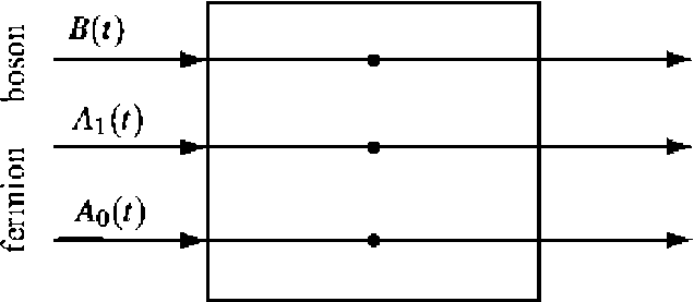
Figure A1.1. Schematic representation of a system coupled to boson B and fermion A, A fields

Some basic aspects of quantum stochastic integrals and the quantum Ito rule are discussed in Appendix A1.2.

The boson field channel B in Figure A1.1 is defined on a symmetric Fock space F . The commutation relations for the boson field are ^ b ( t ) , b * ( t ' ) J = 5 ( t — t ') , from (A1.1). For a boson channel in a Gaussian state, the following singular expectations may be assumed:

(b * (t) b (t ')) = N5 (t — t'),   (b (t) b * (t')) = (N +1) 5 (t — t'),

(A1.3)

(b ( t ) b ( t '^ = M5 ( t — t ') ,    bb * ( t ) b * ( t ')) = M *5 ( t — t ') ,

Here X is a standard notation used to denote the quantum expectation of a system operator X (i.e., {X^х] = E [ X ] , N >  0 is the average number of bosons, while M describes the amount of squeezing in the field state. We have the identity | M |²<  N ( 1 + N ) . For a thermal state, M = 0 and

N =

ee( E—ц) _ 1

(A1.4)

where в =---- is the inverse temperature, E is the energy, and ц is the chemical potential.

^k B ^T

We will assume N = M = 0 , which corresponds to the case of a boson field in the vacuum (ground) state. The vacuum boson field is a natural quantum extension of white noise, and may be described using the quantum Ito calculus. In this calculus, the integrated field processes B ( t ) = j b ( s ) ds (annihilation), B * ( t ) = j b ’ ( sds (creation) and Л ( t ) = £ b * ( s ) b ( s ) ds (conservation) are used. The non-zero Ito products for the vacuum boson field are

d Л( t) d Л( t) = d Л( t), d Л( t) dB * (t) = dB * (t), dB (t) d Л( t ) = dB (t), dB (t) dB *( t ) = dt

We now specify the fermion channels A and A in Figure A1.1. We assume the followings singular expectations for a fermion field A , defined on an antisymmetric Fock space F :

( a * (t) a (t')) = N5 (t — t'),   (a (t) a * (t')} = (1 — N) 5 (t — t'),

.                (A1.6)

( a (t) a (t ')} = M5 (t — t'),   (a *( t) a *( t')) = M *5 (t — t')

In general we have 0 < N < 1 along with the identity |M| < N(1 — N) . For a thermal state we have M = 0 , and

N =

e ^{e ( E —} ^ ) + 1

(A1.7)

In what follows we take the zero temperature limit T ^ 0 . For fermion channel 1 we assume the energy is such that E < ц and so in the zero temperature limit this channel is fully occupied, N = 1, and the Ito rule dA,*(t) dA (t) = dt (A1) applies for the corresponding integrated processes A (t) = JQ a\ (s) ds and A’ (t) = j^!’ (s) ds. For fermion channel 0 we fix E > ц, in which case N = 0, describing a reservoir which is unoccupied. The number process Ло (t) = £а0' (5) a0 (s) ds (but not for channel 1), and the Ito table is is well defined for fermion channel 0

dЛо (t) dЛо (t) = dЛо (t), dЛо (t) dA (t) = dA0 (t), dA (t) d Ло( t ) = dA (t), dA (t) dA 0( t ) = dt

(A1.8)

( 1 )                ( 0 )

The fermion channels are defined on distinct antisymmetric Fock spaces F , F     .

System Coupled to Boson and Fermion Fields

The system S illustrated in Figure A1.1 is defined on the Hilbert space Y , and so the complete system coupled to the boson and fermion fields is defined on the tensor product Hilbert space

Y = Y s® F m ® F(^  ® F**                          (A1.9)

S     sym      antisym      antisym

Due to the presence of fermion field channels, it is necessary to introduce a parity structure on the collection of operators on this tensor product space. We therefore have a parity operator т on Y such that for all operators X and У on Y we have т ( XY ) = т ( X ) т ( Y ) and т ( X ^o ) = т ( X ) . Operators X such that т ( X ) = X are called even , while those for which т ( X ) = — X are called odd . As example, fermion annihilation and creation operators are odd, while the fermion number operator is even. All boson operators are even. A system operator, i.e. an operator X acting nontrivially on Y only, that is even will commute with all field operators, while an odd system operator will anticommute with odd fermion field operators. All boson field operators commute with all system operators and all fermion field operators.

The Schrödinger equation for the complete system is

dU(t) = ^(S — I)dЛ(t) + dB*(t)L — LSdB(t) — jLLdt + dA*(t)A — L\dAx (t) — j LLOddt^U(t) + ((So — I) dЛо (t) + dA: (t) Lo — L0SodA (t) — j L0Ldt — iHdt ^ U (t)               (A1.10)

with initial condition U (0) = I. The operators S, L, H, So, L and Lo are system operators, where o S, L, H, S are even (and thus also their adjoints), and o L and L are odd (and thus also their adjoints).

The operator H is called the Hamiltonian, and it describes the behavior of the system in the absence of field coupling. The operators S , L , H , S , L and L describe how the field channels couple to the system ( S and S are required to be unitary). Note that often terms involving the creation and annihilation operators in (A1.10) ensure a total energy conserving exchange of energy between the system and the field channels; for example, an electron may transfer from the field to a quantum dot, and vice versa. Consequences of the specified parity of the above operators and the fact that U ( 0 ) = I is even is that U ( t ) is even and hence commutes with all the Ito differentials, and, by the quantum Ito rule, is a unitary process (we have dA 0 L_o = — L_odA 0 , dAL = — AdA , and dB ^o L = LdB ^o , .

Heisenberg Picture Dynamics

A system operator X at time t is given in the Heisenberg picture by X ( t ) = j ( X ) = U ( t ) XU ( t ) and it follows from the quantum Ito calculus and the commutation and anticommutation relations arising from the chosen parity that

dj, (x ) = jt (S * XS - X) d Л( t) + dB (t )* j (S *[ X, L ]) + j ([ L*, X ] S) dB (t) + j (L (X)) dt+ dAi (t ); jt (т (X) Li - LX) + jt (LT (X)-XL) dAi (t) + jt (L1 (X)) dt

(A1.11)

+ j _t ( S , XS о - X ) d Л о ( t ) + dA ( t ) * j _t ( S , ( т ( X ) L о - L ₀ X ) )

+ j, ((L0t(X)-XL0)Sо)dAо (t) + jt (Lo (X))dt-it ([X,H])dt where

L ( X ) = LXL - 1 XLL - 1 LLX , L ( X ) = L T ( X ) L ; - 1 XLL - 1 LLX ,

( X ) L о - 1 XL , L о - 1 L , L о X ,

L o ( X ) = L 0

т and in the case of even operators we shall just write

L , ( X ) = l ; t ( X ) L , - 1 XE . L, - 1 E . L . X , ( I = О,1 ) .

The boson and fermion output fields are defined by

Bout (t) = U;(t)B(t)U(t),  Л„,t(t) = U;(t)Л(t)U(t), A,,out (t) = U;(t)A (I)U(t),A,out (,) = U;(I) A (t)U(t), Ло,out (t) = U;(t)Ло (t)U(t)

and satisfy the corresponding quantum stochastic differential equations (QSDEs)

dBo„ (t) = j, (L)dt + j, (S)dB(I), dЛo„ (t) = jt (LE^dt + dB;(t) jt (S;L) + j, (ES)dB(t)+dЛ(t), dAt««, ( t ) = j, ( L1 ) dt + dA1 (t ), dA0,out ( t ) = j, ( Lо ) dt + j, ( Sо ) dA0 (t ), d Ло„ (t) = j, (^о L о) dt+dA,• (t) j, (Sо Lо)+j, (Eo Sо) dA, (t) + d Ло (t)

The State

Let us define a state E [ . ] on the von Neumann algebra of observables to be an expectation, that is, a linear positive normalized map from the observables to the complex numbers; positive meaning that E ^ X ^; X J >  О for any observable X and normalized meaning E [ I ] = 1 , where I is the identity operator. For technical reasons we require the state to be continuous in the normal topology. We shall assume that the state is a product state with respect to the system-environment decomposition: E [ X ® F ] = ( X)_s (F )₅, for system observable X and environment observable F . In particular we take 0_£ to be the mean zero gaussian state with covariance (A1.6) and the choice of N = 1 (the Fermi vacuum).

We say that the state is even if we have

E о т = E ,                                     (A1.12)

where т is the parity operator that was introduced above. Specifically, this forces all odd observables to have mean zero. In quantum theory, the observable quantities must be self-adjoint operators, however, it is not necessarily true that all self-adjoint operators are observables as there may exists so-called superselection sectors. In the present case, only the even self-adjoint operators are observables. We need to ignore states which lead to unphysical correlations between component systems, this is referred to a superselection principle in the quantum physics literature. We need therefore to restrict our interest to even states only. More specifically, we shall assume that the factor states 0 and 0 are separately even on the system and environment observables respectively.

The expected values of system operators X evolve in time as follows. Define

Л ( X ) = E [ j, ( X ) ]                               (A1.13)

Then by taking expectations of (A1.11) we find that for even observables X

A t ( X ) = _{M t} ( L ( X ) + L , ( X ) + L o ( X ) ) ,                      (A1.14)

which is called the master equation , and corresponds to the Kolmogorov equation. This may be expressed in Schrodinger form using the density operator p (t ) defined by p_t ( X ) = Tr [ p ( t ) X ] which exists by our assumption of normal continuity of the state. The density operator is then an even positive trace-class operator, normalized so that Tr [ p ( t ) ] = 1 , satisfying the equation

p( t) = L ( p (t))+Li ( p( t))+L0 ( p ('))                        (A1.15)

where

L ' ( p ) = L p C — 1 LL p — 1 p LL ,

l;( p) = l pL,

—

1 LL P

—

1 p ll ,

^L0 ^{( p )} = L 0 ^P L 0   2 L ° L o ^{P  рР}^ L o .

Fermion Filter

We suppose that electrons in fermion channel 0, after interaction with the system, can be continuously counted; that is, the observables A_{o out} ( s ) ,0 <  s <  t are measured. The problem is, given an even state E as outlined above, to determine estimates J X ( t ) of system operators X given the measurement record. This is a filtering problem involving a signal derived from a fermion field. As mentioned above only the even operators may be observable, and in fact the expectation and conditional expectation of all odd operators must vanish identically. Mathematically, we wish to determine equations for the quantum conditional expectations

XX(t) = п,(X) = E[jt(X)J t]

(A1.16)

Here, X is a system operator, J _t is the algebra generated by the operators Л_{о out} ( s ) ,0 <  s <  t , a commutative von Neumann algebra, and п is the conditional state. In quantum mechanics, conditional expectations are not always well defined due to the general lack of commutativity. However, the conditional expectation (A1.16) is well defined because j_t ( X ) commutes with all operators in the algebra J _t . This is called the non-demolition property, and is a consequence of the system-field model, where fermion field channel 0 serves as a probe. The quantum conditional expectation (A1.16) is characterized by the requirement that

E [ j_t ( X ) Z ] = E [ п ( X) Z ] for all Z e J _t                   (A1.17)

The quantum filter for the conditional expectation (A1.16) is given by п ( X ) = 0 for odd observables, while for even observables satisfies the equation

dn ( X) = п

(- i [ X, H ] + L (X ) + L ( X) + Lo ( X )) dt

п ( Lo XL0 ) Kt ( Lo Lo)

- п ( X H dW ( t ) (A1.18)

where W ( t ) is a J , martingale (innovations process) given by

dW (t) = dY (t)- п (LLo) dt, W ( 0) = 0.

Let p be the initial even density matrix for the system, then in the Schrodinger picture we may define the conditional density operator p ( t ) by п ( X ) = Tr [ p ( t ) X J , and obtain the filtering equation

d p (t ) = ( L°( p (t))+L°( p ( t ))

^{+ L}0 ( ^p ( t ) ) ) ^dt

+ <

L 0 P ( t ) L 0

„ Tr (L„ p (t) L0)

- p ( t H dW ( t ) .

Appendix 2. Quantum stochastic calculus

Let B, = { B_t ( to )| to e Q } , t >  0 , be one-dimensional Brownian motion. Integration with respect to B, was defined by Ito. A basic result of the theory is that stochastic integral equations of the form

X = X 0 ¹ 1 t b ( s ' X . ) ds + i, t c ( s , X . ) dB .                        (A2.1)

can be viewed as stochastic differential equations of the form dXt = b (t, Xt) dt + cr (t, X,) dB,                              (A2.2)

where differentials are handled with the use of Ito’s formula

( dB, ) 2 = dt , dBdt = dtdB, = ( dt ) 2 = 0 .                        (A2.3)

Hudson and Parthasarathy obtained a Fock space representation of Brownian motion and Poisson process.

The Boson Fock space Г = r(L2 (□ +, C)) over L2 (□ +, C) is the Hilbert space completion of the linear span of the exponential vectors ^ (f)under the inner product ^ (f) ,^ (g)^ = e^f,g, where f, g e L (□ + , C) and ff, g^ = J f (s) g (s) ds where, here and in what follows, z denotes the complex conjugate of z e □ .

The annihilation, creation and conservation operators A ( f ) , A ⁱ ( f ) , and Л ( F ) respectively, are defined on the exponential vectors V ( g ) of Г as follows.

.V ^{( g + T} Z _M) ^; Л ^ ^{( g}^

V ( e ’‘'“'g ) •

Av (g ) = Jotg (s) dsv (g); Av (g ) = ^ 0                           dm

The basic quantum stochastic differentials dA_t , dA_t and d Л^ are defined as follows.

dA , = A + « - A , ; dA , = A, + , - A, ; d Л, = Л, +, - Л, •

The fundamental result which connects classical with quantum stochastics is that the processes B and

P defined by B_t = A + A ; P = Л, + V X ( A + A i ) + X t are identified through their vacuum characteris-

- ¹ S 2

tic functions V ( 0 ) , e^lsB‘v ( 0 )) = e ²

V V ( 0 ) , e^iP* V ( 0 )} = e ^X e i ^{- 1 )} )

with Brownian motion and Poisson

process of intensity X respectively.

Hudson and Parthasarathy defined stochastic integration with respect to the noise differentials of definition and obtained the Ito multiplication Table

-	dA^t	dXt	dAt	dt
t/л;	0	0	0	0
dXt	^	dXt	0	0
dA,	dt	dAt	0	0
dt	0	0	0	0

Within the framework of Hudson-Parthasarathy “Quantum Stochastic Calculus”, classical quantum mechanical evolution equations take the form dU = iH + -L L dt + L HdAt - LdAtf +(I - W) d Л, Ut; Uo = I,

(A2.4)

t    2        .......

where, for each t >  0, U_t is a unitary operator defined on the tensor product H ® Г ( L (□ ₊, C ) ) of a system Hilbert space H and the noise (or reservoir) Fock space • Here H, L, W are in B ( H ) , the space of bounded linear operators on H , with W unitary and H self-adjoint. In all cases, I denotes the appropriate identity operator. Here and in what follows we identify time-independent, bounded, system space operators X with their ampliation X ® I to H ® r ( L (□ ₊, C ) ) . All Hilbert space inner products are linear on the right.

The quantum stochastic differential equation satisfied by the quantum flow j_t ( X ) = U * XU_t , where X is a bounded system space operator, is

Электронный журнал «Системный анализ в науке и образовании»

d., ( X ) = j_t ^ i [ H , X ] — 1 ( LLX + XL*L — 2 L*XL ) ^| dt

+ j, ([С,X] W)dA + j, (W•[X,L])dA/ + j, (W• XW —X)dЛ,, jо (X ) = X, t e[0, T ]

The commutation relations associated with the operator processes A , A ^† are the Canonical (or Heisenberg) Commutation Relations (CCR), namely ^ A , A ^L J = I .

Elements of quantum stochastic differential equations

In the previous sections, we derived equations of motion for single and cascaded components interacting with probe fields, which produce dynamics when integrated. It turns out, however, that proper integration is far from trivial, not just because the dynamics are complex, but because they are inherently stochastic. In this section we will summarize the use of Ito calculus to calculate these stochastic quantum dynamics.

So far, we have been fairly cavalier (nevertheless, accurate) about dealing with the broadband input fields b_in ( t ) . The mathematical description of these fields is highly singular due to the canonical commutation relations ^ b_in ( t ) , b ^L ( t ') ] = 5 ( t — t ') . To sidestep such singularities, let us define the time-integrated quantities B_in ( t ) = J b_in ( s ) ds and B ^L ( t ) = J b ^L ( s ) ds , and consider increments in these fields dB_in ( t ) = J b_in ( s ) ds , d B ^L ( t ) = J b L ( s ) ds . Note that the units of these increments are Vtime , and their commutation relations are ^ dB_in ( t ) , dB ^L ( t ') J = dt for t = t ' and zero otherwise. These are quantum, non-commuting analogues of the classical Wiener process and are referred to as quantum noise increments or quantum stochastic increments .

Further, by using the above singular commutation relations we can compute the following vacuum expectation values ddB.. (t)dB„ (t')) = 0,   (dB* (t)dB* (t')) = 0, for t = t', and zero otherwise,

(dB' (t)dB,. (t')) = 0,  (dB, (t)< (t')) = dt, where ^A^ = Tr (pin A) and pin is the initial state of the asymptotic input field, which is assumed to be the vacuum state of all frequency modes. The vacuum expectation values above are somewhat surprising because they state that the average value of second order products of increments of the input fields can be proportional to a first-order time increment (dt) . This bears resemblance to stochastic Wiener increments in classical stochastic theory, and motivates us to think more deeply about how to integrate over such increments. Similar to classical stochastic increments, we define two types of integrals over the quantum stochastic increments dBin (t) :

• n — 1

• (    I) J0 g (s )dBn (s ) = lim E g (ti ) [Bin (ti +1 ) — Bin (ti )] ,

i = 0

n — 1

• (S) Jo g (s)dBin (s) = lim E g I A (ti+1 + ti ) I [Bin (ti +1 ) — Bin (ti )],

i = 0    \ ²            7

where the time interval [ 0, t ) has been discretized into n segments, and g is any operator in the system subspace. These two definitions of integration, the first of which is called an Ito integral and the second is called a Stratonovich integral, are equivalent in standard calculus where the increments are regular. However, since the quantum stochastic increments can vary wildly even in the n →∞ limit, these two integral definitions produce different results. As such, one must specify the type of integral a quantum stochastic differential equation (QSDE).

In general, a QSDE derived from physical principles (e.g. Heisenberg equations of motion) corresponds to the Stratonovich integral definition. To understand why this is, note that real physical noise is never exactly a white noise process. Instead, one uses (classical or quantum) white noise as an approximation of a real physical process in some limit (e.g. white noise approximates the Ornstein-Uhlenbeck process in the vanishing correlation time limit). The Wong-Zakai theorem, and its quantum generalization, state that the behavior of a noise-driven physical system under this singular approximation of the real noise process is captured by a QSDE that is interpreted with respect to Stratonovich integration. This is consistent with the fact that Stra-tonovich differentials are consistent with standard calculus rules, while Ito differentials obey a modified chain rule:

d ( X ( t ) Y ( t ) ) = dX ( t ) Y ( t ) + X ( t ) dY ( t ) + dX ( t ) dY ( t ) , (А2.5) where X ( t ) and Y ( t ) are arbitrary functions of operator valued stochastic variables and dX ( t ) and dY ( t ) are specified in terms of Ito QSDEs. The first two terms arise from the usual non-commutative chain rule and the third term is known as the “Ito correction".

Therefore, the QSDEs we derived in the previous section for system operators or unitary propagators should be interpreted with respect to the Stratonovich integral (or more succinctly, we will refer to QSDEs being in Stratonovich or Ito “form"). However, QSDEs in Ito form are often much easier to work with analytically and numerically. Fortunately, there is a straightforward procedure to convert between QSDEs in Stratonovich and Ito forms.

In much of the following, an important mathematical object will be the unitary propagator for the system, which generates evolution of any system operator (in the Heisenberg picture), a ( t ) = U ^t ( t ) aU ( t ) . For the dynamics described above, the propagator takes the form:

U ( t ) = T exp {£ ^ds ( ^- iH sys + ( Lb_R ( s ) ^- Lb in ( s ) ) ) } , with ^U ( t 0 ) = I SF . (A2.6)

Here T denotes time ordering, I is shorthand for the identity operator on the system and field degrees of freedom (i.e. I _tem ® I^_ш\ and we introduce the coupling operator L = YC^c (note that while L is commonly referred to as an operator, it has units of time -^ ). One calculates the generator of this unitary, K ( t ) , as

U (t ) = K (t) U (t ) = [-iHs, +(Lbin (t)-Lbn (t))] U (t).                 (A2.7)

Because it will be used heavily in later sections, we write the Ito form here dU (t ) =

iHsvs +1 LfL | dt + LdB^ - Lf dBin sys 2         ।                in             in

dU ( t ) , with U ( 0 ) = I_{s F},

(А2.8)

where the term LLdt arises from the conversion between Stratonovich and Ito forms (i.e. the Ito correc- 2

tion).We will often write the Ito propagator U ( t ) as U_t for convenience.

Remark . [QSDE notation] By convention, QSDEs in Ito form are nearly always written in terms of increments (e.g. an equation for dU ( t ) and not dU ( t ) / dt ). Stratonovich QSDEs are also sometimes written in terms of increments and in that case, it is customary to make explicit the Stratonovich interpretation by writing the product of a (possibly operator-valued) quantity g ( t ) and an increment B ( t ) as: g ( t )o dB ( t ) .

Applications of quantum stochastic calculus to the control of quantum evolutions and Langevin equations (quantum flows) can be found and the references within it. However, to the author’s best knowledge, no work has been done in the direction of performing actual numerical computations, most likely with the use of a computer [8]. That would require the implementation of suitable algorithms whose reliability depends on the existence of good norm estimates. It is that gap that this Appendix 2 aspires to close.

Appendix 3: Ito and Stratonovich calculus

Definitions of the Ito and Stratonovich multiplications for arbitrary stochastic operators X and Y in the Schrödinger representation are given, respectively, by

dX t • Y = ( X . + dt - X, ) Y                                (A3.2)

and x.-dY, = 1 (X.. dt + x,)( Y+d. - Y),                          (A3.3)

dX.«Y = (X „ d - x,) 1 ( Y + d + Y ) .                       (A3.4)

From these relations we have the connection formulae between the Ito and Stratonovich products in the differential form as

XodY = X • dY + ¹ dX, • dY ,                         (A3.5)

dX o Y = dX_t • Y + ¹ dX • dY .                          (A3.6)

Note that random average of the stochastic multiplication (A3.1) or (A3.2) of the Ito type is equal to zero.

Definitions of the Ito and Stratonovich multiplications for stochastic operators X ( t ) and Y ( t ) in the Heisenberg representation are given in the same form by

X (,)• dY (t) = X (t)[y (t+dt)-Y (t)],                         (A3.7)

dX (t )• Y (t ) = [ X (t + dt)-X (t)] Y (t),                         (A3.8)

and

X (t )o dY (t ) = 1 [ X (t + dt) + X (t )][Y (t + dt)-Y (t)],                (A3.9)dX (t )o Y (t ) = [ X (t + dt)-X (t)] 1 [Y (t + dt) + Y (t)],                (A3.10)

where operators X ( t ) and Y ( t ) are introduced, respectively, through relations

X ( t ) = V ^ ( t ) X^ ( t ) ,                              (A3.11)

dX ( t ) = d ( V / ( t ) X^ ( t ) ) ,                          (A3.12)

with V _F ( t ) being a stochastic time evolution operato r.

From (A3.7) to (A3.10), we have the connection formulae between the Ito and Stratonovich products in the differential form as

X ( t ) о dY ( t ) = X ( t ) • dY ( t ) + 1 dX ( t ) • dY ( t ),                       (A3.13)

dX ( t ) о Y ( t ) = dX ( t ) • Y ( t ) + 1 dX ( t) • dY ( t ) .                      (A3.14)

Stochastic multiplications (A3.7) to (A3.10) are consistent with corresponding types of differential calculus for products of stochastic operators, which for the case of the Ito type calculus and the Stratonovich type calculus read, respectively, as

d [ X (t) Y (t )] = dX (t )• Y (t) + X (t) dY (t) + dX (t )• dY (t),             (A3.15)and d[X(t)Y(t)] = dX(t)oY(t) + X(t)odY(t).