Some interrelations in matrix theory and linear algebra for quantum computing and quantum algorithms design. Pt.2

Matrices have been the subject of much study, and large bodies of results have been obtained about them. In this article we introduce main definitions of matrix theory and study the interplay between the theory of matrices and the theory of orthogonal polynomials in quantum computing [1-7]. Interesting results have been obtained for Krawtchouk polynomials and also for generalized Krawtchouk polynomials. More recently, it was obtained conditions for the existence of integral zeros of binary Krawtchouk polynomials. Also it was obtained properties for generalized Krawtchouk polynomials. Other generalizations of binary Krawtchouk polynomials have also been considered. Generalized some properties of binary Krawtchouk polynomials to q-Krawtchouk polynomials, derived orthogonality relations for quantum and q-Krawtchouk polynomials and showed that affine q-Krawtchouk polynomials are dual to quantum q-Krawtchouk polynomials. In this paper, we define and study a generalization of Krawtchouk polynomials, namely, m-polynomials [8-11]. Applications of Krawtchouk / Hadamard matrices in quantum algorithm’s design are considered.

Krawtchouk matrices and quantum random walk

In quantum probability, random variables are modelled by self-adjoint operators on Hilbert space and independence by tensor products. We can model a symmetric Bernoulli random walk as follows. Consider a 2-dimensional Hilbert space V = R1 and two special 2 x 2 operators satisfying F2 = G2 = I, the 2 x 2 identity. Recall the fundamental Krawtchouk/Hadamard matrix H (see, Part 1, Eqs (2) and (4)), which we shall now view as

H = F + G =

( 1   1 1

1 1   —

One can readily check that

FH = F ( F + G) = ( F + G) G = HG

(use F ² = G ² = I ). This, of course, can be viewed as the spectral decomposition of F and we can interpret the Hadamard matrix as diagonalizing F .

Remark . Note that the exponentiated operator

exp ( zF ) =

^л cosh z _v sinh z

sinh z cosh z >

has the expectation value in the state e equal e e0 ,exp (zF) e0 ^ = cosh z which coincides with the moment generating function for the symmetric Bernoulli random variable taking values ±1. This shows that indeed we are dealing with the (quantum) generalization of the classical model.

Remark. ( Quantum computing interpretation ). We can view V = span { e ₀, e_x } as a Hilbert space representing a simple two-state quantum system, e.g., a particle with possible spin-up ( e ) and spin-down ( e ) states, respectively. In the context of “quantum computing”, these elementary states represent “qubits”. The operator F represents a “spin flip” and G a “phase change”, both are thus basic qubit operations. Geometrically, they are reflections in V through lines that form 45 degrees. The Hadamard matrix M is essentially a “rotation by 45 degrees” (up to composition with reflection and scaling) and therefore ties them via (1). Now, to perform quantum computing, one needs an assembly of N such independent systems – this constitutes a simple quantum computer. The Hilbert space of computer states is represented by the N -th tensor product of the original space V , that is, by the 2 N -dimensional Hilbert space V ⁰ N . This motivates our further considerations.

Define the following simple operators (cf. Appendix 1) f = F 0 1 0-0 1

f = 1 0 F 0 1 0-0 1

fN = 1010-0 F each f describing a “flip” at the i -th position. These are our quantum equivalents of the random walk variables. Performing them independently would result in “running” a classical TV-bit computer. We shall consider the superposition of these independent actions, setting

X f = f + - + f N-

Notation : For notational clarity, since N is fixed throughout the discussion, we drop N indices on X ’s.

Analogously, we define:

g = G 0 1 0...01

g₂ = 1 0 G 0 1 0---0 1

g_N = I 0 I 0-0 G

With XG = g1 +-----+ gN. We also extend H to the N -fold tensor product, setting HN = H0N. (This is the same as H( ) of the previous sections.)

For illustration, consider a calculation for ^N = ³ :

fH =( F 0 I 0 I)( H 0 H 0 H )= (H 0 H 0 H)(G 0101) = Hg where the relation FH = HG is used. This clearly generalizes to fkHN = HNgk and, by summing over k , yields an important relation:

X f H n = H n X g .

Since products are preserved when reducing to the symmetric tensor space, we get

XFHN = HNXG the bars indicating the corresponding induced maps (see Appendix 2). We know how to calculate H from the action of H on polynomials in degree N . Note that for symmetric tensors we have the components xN-kxk in degree N for 0 < k < N .

Proposition. For each N >  0 , symmetric reduction of Hadamard matrices leads to H. = Ф ^{( N} ) That is, ij            ij

H_N is the transpose of the Krawtchouk matrix Ф ^{( N} ) .

Proof: Writing ( x, y ) for ( x ₀, x _t) , we have in degree N for the k ^th component:

( x + y)N-k ( x - y )k = £ HkiXN-ly1 .

l

Scaling out x ^N and replacing и = y / x yields the generating function for the Krawtchouk matrices with the coefficient of u¹ equal to Ф ⁽ _lk ^N ) . Thus the result.

Now consider the generating function for the elementary symmetric functions in the quantum variables f . This is the N - fold tensor power

Fv (t ) = ( I + tF )0 N = 10 N + tXF +- noting that the coefficient of t is X . Similarly, define

QN (t ) = ( I + tG )0 N = 10 N + tXG +■■•

(I + tF ) H = H (I + tG )

From                     we have

^XN^HN = ^HN^N and N H I = = ^Hn^N .

The difficulty is to calculate the action on the symmetric tensors for operators, such as X , that are not pure tensor powers. However, from X_N ( t ) and N _n ( t ) we can recover X_F and X_G via

Xf = d-   (I + tF )0 N, dt t=0

d XG = — dt

/ _T       0 N

( I + tG )

t = 0

with corresponding relations for the barred operators. Calculating on polynomials yields the desired results as follows:

In degree N , using x and y as variables, we get the k th component for X and X via d dt

(x + ty ) N k (tx - y ) k = ( N - k ) x t=0

. ^N - ( ^k + 1 ) y k + 1

+ kx" ^{-( k - 1 )} y k ^{- l}

and since I + tG is diagonal,

d dt

(1 +1) N" k (1 -1) kx" -kyk t=0

( N - 2 k ) x " - ^k y ^k

For example, calculation for N = 4 result in

Xf =

( 0

4  0  00

0  3  00

2  0  20

0  3  01

0  0  40

	( 1	4	6
	1	2	0
H 4 =	1	0	- 2
	1	- 2	0
	v 1	- 4	6

4    1 ^

- 2   - 1

0    1

2    - 1

- 4   ¹ V

	" 4  0  0   0   0 " 0  2  0  0   0
X g =	0  0  0   0   0 0  0  0   - 2  0 v 0  0  0   0    - 4 V

We observe the spectrum of X _N is N , N - 2,..., 2 - N , - N , which coincides with the support of the classical random walk .

We note that the top row of

^ ^{N      ( k} )         w ( k )

is t where       is the binary shuffling function of section

3. This is seen by noting that each time one tensors with I ^{+ tF} , the original top row is reproduced then it is concatenated with a replica of itself modified in that each entry picks up a factor of t . Now, collapsing to the

k symmetric tensor space, the top row will have entries ^ V

t ^k

. This follows as well by direct calculation of

( x + ty ) "

the 0th component matrix elements in degree N , namely by expanding

.

To find the distributions, we must calculate expectation values. In the present context, expectation values in two particular states are especially interesting. Namely, in the state e0 and the normalized trace – the uniform distribution on the spectrum. In the N -fold tensor product, we want to consider expectation values in the “ground state”            and normalized traces. Then we can go to the symmetric tensors. Since exp (zXN )•                    I000...0)

everything factors, one easily obtains the expectation value of          ^N in the ground state            to

,  (coshz)N        ж ж exp(zF) = 2coshz.       trexp(zXF) = 2N (coshz)N .  - be            . For the trace, tr                      implies           F                  and, after normal-

(cosh z)N izing, this yields             .

For the barred operators, we consider the symmetric trace. Here we can use the symmetric trace theorem, detailed in Appendix 2. It tells us that the generating function for the symmetric traces of any operator

• det ( I - tA )—‘        _ A = exp ( zF )

A in the various degrees is               . Taking               , we have det (I - tezF )-1 = [(1 - tez ) (1 - te"z)]-'

= ( 1 - 2t cosh z + 1 ² )   .

The latter is the generating function for Chebyshev polynomials of the second kind, so that the normalized symmetric trace is

( N + ¹ ) ^{- 1}tr N_m exp ( zF ) = U N ( cosh z ) / ( ^N + 1 ) .

This equals as well

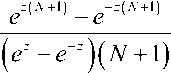
and that completes this study.

A A ® ^N

If A is represente d by a matrix, given the matrix form ^N        computed as an ^N -fold Kronecker

A product, to reduce to N , we see that acting on polynomials, for a fixed row label in the full tensor space, the column entries corresponding to basic tensors equivalent under permutation are summed to a single column. Then the matrix elements are chosen, one row from each equivalence class of basic tensors. What if d 2? Then row and column labels are single indices so that AN is an matrix with

labels according to the exponent of x1 . That is, the basis for polynomials in degree N is given by the mo-XN-kxk nomials 0   1 , 0 - k - N . The binary shuffling function and contraction operations are exactly the reduc tion to symmetric tensors and then induced matrix, (see Table 1 and 2) respectively.

Table 1: Krawtchouk matrices

Ф ⁽⁰⁾= [ 1 ]

Ф (³) =

Ф w

- 1

- 1

1   - 1

- 1

- 1

Ф ^{( 2 )}= 2

0   - 2

- 1

4  2   0  -2

"3  ф(4)= 6   0   -2   06

4  -2  0   2

-1

J     1 -11

Ф ( 5 ) =

Ф ( 6 ) =

- 2

- 3

- 1

- 2

- 2

- 1

- 2

- 1

- 3

- 3

- 5

- 10

- 1

5    - 1

- 5

- 1

- 4

- 1    1

0  -2  -4

-3  -1   515

0   4   0

3   -1  -515

0 -24

-11  -11

5 ⁽⁰⁾=[1]

Table 2: Symmetric Krawtchouk matrices

- 1

5 (2) = 2

0   - 2

- 2

5(3) =

3   - 3   - 3

- 3   - 3  3

1 - 33   - 1

	"1    4     6     4    1 " 4  8    0    - 8   - 4
5 (4) =	6  0    - 12   0   6 4   - 8   0    8   - 4 1   - 4   6    - 4   1

	■ 1	5	10	10	5	1
	5	15	10	- 10	- 15	- 5
5 151 =	10	10	- 20	- 20	10	10
	10	- 10	- 20	20	10	- 10
	5	- 15	10	10	- 15	5
	1	- 5	10	- 10	5	- 1

	■ 1	6	15	20	15	6	1
	6	24	30	0	— 30	— 24	— 6
	15	30	— 15	— 60	— 15	30	15
S (6) =	20	0	— 60	0	60	0	— 20
	15	— 30	— 15	60	— 15	— 30	15
	6	— 24	30	0	— 30	24	— 6
	_ 1	— 6	15	— 20	15	— 6	1

Let us consider the relationship between the structure of Simon’s algorithm and Walsh transforms.

Entropy and Hadamard matrices

We will define the entropy of an orthogonal matrix. It provides a new interpretation of Hadamard matrices as those that saturate the bound for entropy. This definition play important role in QAs simulation, while the Hadamard matrix is used for preparation of superposition states and in entanglement-free QAs. We define the entropy of orthogonal matrices and Hadamard matrices (appropriately normalized) saturate the bound for the maximum of the entropy. The maxima (and other saddle points0 of the entropy function have an intriguing structure and yield generalizations of Hadamard matrices.

Consider n random variables with a set of possible outcomes i = 1,..., n having probabilities pt, n                                                Sh             n г = 1,...,n. We have Lp( = 1 and the Shannon entropy S (p) = —Lp{ Inpt .

i = 1

i = 1

We now define entropy of an orthogonal matrix O p i , j = 1,... , n . Here Oi are real numbers with the constraint 'L1O ⁱ Oⁱ_k = 5_k . In particular, the j th row of the matrix is a normalized vector for each i = 1

i = 1,..., n . We may associate probabilities p(i) = (Oi ) with the i -th row, as L pj) = 1 for each i. We j \ j /                                        j=1 j define the Shannon entropy for the orthogonal matrix as the sum of the entropies for each row:

S '* ( O h—i: ( O j ) ² in ( o )¹ .

i , j = 1

The minimum value zero is attained by the identity matrix O i = 5\ and related matrices obtained by interchanging rows or changing the signs of the elements. The entropy of the i -th row can have the maximum value In n , which is attained when each element of the row is ± —U-. This gives the bound,

S S ( O, ) < n in n .

In general, the entropy of an orthogonal matrix cannot attain this bound because of the orthogonality

L OO = 5 _{jk              p} (i )

constraint i=1             , which constraints Fj for different rows. In fact the bound is obtained only by the Hadamard matrices (rescaled by n ). Thus we have the criterion for the Hadamard matrices (appropriately normalized): those orthogonal matrices which saturate the bound for entropy.

Remark. The entropy is large when each element is as close to possible, i.e., to a main diagonal.

±  ‘

n

Thus maximum entropy is similar to the maximum determinant condition of the Hadamard. The peaks of the entropy are isolated and sharp in contrast to the determinant.

Example. Matrix that maximizing the entropy for n = 3 is
	(   1	2	2 >
	— 3	3	3
	2	1	2
	3	— 3	3
	2	2	1
	13	3	— 3 )

For n = 5 , the result is similar: the magnitudes of the elements in each row are — repeated 4 times and

3  _ .          ,          _   , „          _        .    _ n - 2  ,     , a diagonal element is a —. This set can be generalized for any n . The matrix with--along the diag-

5n onal and each off-diagonal as is orthogonal. Each row is normalized as a consequence of the identity: n

n2 = ( n - 2 )2 + 22 ( n -

For each n , there are saddle points apart from maxima and minima.

Example . For n = 3 there is a saddle point and the corresponding matrix is
	" 1      1      1 "
	222
	1       ~          1
	0   —1=	.
	22
	111
	v 2   - ^2    2 ,

The entropy peaks quite sharply at all extrema. Thus the entropy has a rich set of sharp extrema.

This result shows the important role of Hadamard operator in entanglement-free QA: with Hadamard transformation it is possible introduce maximal hidden information about classical basis independent states and superposition includes this maximal information. Thus, with superposition operator is possible created a new QA without entanglement while in any cases superposition includes information about the property of function f .

General properties of Walsh-Hadamard transformation w (a, b, q). (see Appendix 3)

Let us consider a function W : Л/'хЛ/'х{ 2 ⁿ|n eZ⁺}^{- 1,1 } . The function satisfies the following conditions:

W ( 0, b, q ) = 1 W ( a Ф c, b, q ) = W ( a, b, q ) W ( c, b, q ) W (a, b, q ) = W ( b, a, q ) § W ( a, c, q ) W ( c, b, q ) = q5ab c=o where the operator Ф is a bitwise exclusive-OR (XOR). Moreover, we define the transform Wq as fol lows: | a) ———> —7= X W ( a, c, q )| c^ . When the a -th row and b -th column element of a matrix Uw is V q c=0                                                                                       q

—i= W (a, b, q) (unless otherwise specified, the rows and columns will be indexed beginning with 0), the q matrix is a unitary matrix because of the definition of W (a, b, q). Thus, the Quantum Turing Machine (QTM) can execute the transform W .

Example. Let W (a, b, q = 2n ) = (—1)ab where a • b is an inner product of a and b , i.e., for a = X az 2i and b = X b 2i  at, bt e {0,1}, a • b = X ab (mod 2). Obviously, the function W (a, b,2n)

i = 0                        i = 0                                                 i = 0                                                                    ^{X            7}

satisfies the conditions above of W ( a , b , q ) . In fact, by using W ( a , b ,2 ⁿ ) , in the Simon algorithm

W ( 5 , c ,2 ⁿ ) = 1, 5 • c = 0 .

Next, let us consider the case when W (a, b, q) is a discrete Walsh function. We will show that the function W ( a, b,2n) is a kind of discrete Walsh function.

First, we describe Walsh functions and discrete Walsh functions. We define a function

1,

( x ) : R ^ { - 1,1 } by r ( x ) =

— 1, — <  X <  1

and r ( x + 1 ) = r ( x ) . Moreover, let r_l ( x ) be a function r ( x ) = r ( 2 l x ) , where x e R, l e N . Then, a Walsh function (more precisely, Walsh-Paley function ) W, ( x ) is defined by W _z ( x ) = П r ( x ) ^l k , where k = 0

”

l = X l_k 2 ^k , l k e { 0,1 } .

k = 0

Remark. Every value of the function W, (x) is always a finite value because lk = 0 for k that is sufficiently large (in fact, each value of the Walsh-Paley function is either 1 or — 1). Moreover, when let a e N, b e N, and q e Z+, a discrete Walsh-Paley function is defined by Wa

' b

I q J

.

f b 1

Example . Now, let q = 2 ( n e N) . Then, the function W_a — satisfies the following properties [so

V q J that this function satisfies the properties of W ( a, b, q ) ]:

W a

w

f b 1 vqJ

W " a Ф c

f b

v q J

= W a

( b1I q J

W c

( b

V q J

f b 1 vqJ

= W b

c \

a

I qJ

q ^{— 1}

X W a

f" 1 v q J

W c

(hA

- = q5 ab

vqJ

Namely, a matrix U whose the a -th row and b -th column element is     W qq

' b

I q J

is a unitary ma-

trix. The transform P : | a ) ———>

1 q - 1       I c li \

-j= Z W —  c) correspond to the matrix Up qc=o  a q J                               1

and can be computed in ^q

polynomial time of n .

Example . Let H be

a q -dimensional Hadamard matrix ( q = 2 n ) , that is, when H₂ =

। 1    1

. 1    - 1

then

H q = H 2 ® H q /2 =

q /2

q /2

q /2

q /2 j

. The QTM can execute the matrix —h H_q in O ( n ) time. Further, ^q

when let H_{k y}be the k -th row and j -th column element of H_q then H_{k y} = W_br^

j

I q J

where for

k = Z kt 2 i ( k _z e { 0,1 } ) , br ( k ) = Z k , A i (for a bit string, its reverse order is obtained). The QTM can also execute this procedure in O ( n ) time. Consequently, the QTM can execute the transform P in O ( n ) time.

Relationships among some Walsh transforms n-1        i             (      )

For the value a = Z a,2', a. e{0,1}, let i=0

<

g i ( i = ^0,1

g n - 1 = ^a n - 1

.

[g i = ai+1 ® ai(0 ^ i ^ n - 2)

b

Gray code g ( a ) of a is defined by g ( a ) = Z gi 2 i . Now, when W a ,—

and

H a

b

are dis-

i=0                        v q J           v q J crete Walsh-Paley function and Walsh-Hadamard function, respectively, the relationships among Walsh

f

b

A

functions are W a ,— = W_(A

,               g ( a )

V q J

Ib 1I q J

and H

Ib 1 I q J

= Whi A br ( a )

I b 1

— . Moreover, we can describe them by

V q J

( h\ ,   „

W a , - = ( - 1 )

br ( g ( a ) ) • b

Wa I b | = (-1У

br ( a ) • b

Ha b =(-1)

Simon’s problem and algorithm

Simon (1994, 1997) was the first to show a nice and simple problem with expected polynomial time QA but with no polynomial time randomized algorithm.

The qualitative description of Simon’s problem

A function f : { 0,1 } n ^ { 0,1 } n is given as an oracle, with the promise that there exists an s e { 0,1 } n (known as the “hidden secret”) such that f ( x ) = f ( y ) iff x Ф y = s . Notice that if s = 0 ⁿ , then f is a permutation, and otherwise f is two-to-one function. The problem is to tell if s = 0 ⁿ .

Simon’s algorithm works as follows. One starts with 2 n qubits, separated into two n -qubit registers. Originally one initializes the states to | ф ₀) = |0 n^ |0 n^ . Next, one applies the Hadamard operator to the first register and then the oracle operator | x^ | y ^ H^ | x^ | y ® f ( x )^ . The state becomes

I 4) = -7= El xlf(x)).

2 x

Next, the second register is measured and discarded:

o If s = 0 n , then the measurement result is | ф ₂ ) = | x ) for a random x g{ 0,1 } n ;

o If ^s * ⁰ 0

then the measurement is | Ф 2) = “7= (| x ) +1 x ® s )) for a random ^x 2₂

Next, a Hadamard operator is applied to the first register.

In the case s = 0 n , the result is | Ф 3) = | y ) for a random y ; in the case s * 0 n , the result | Ф з) = | y ) for a random y such that y • s = 0 .

Finally, one measurement the first register and obtain y .

Repeating the experiment O ( n ) times, one can solve for s by using Gaussian elimination and distinguish the case s = 0 ⁿ from the case s * 0 ⁿ .

Mathematical model of Simon’s problem: Simon’s XOR Problem

Let f : { 0,1 } n ^ { 0,1 } n be a function such that either f is one-to-one and there exists a single nonzero s g { 0,1 } n such that V x * x ' ( f ( x ) = f ( x ') ^ x ' = x ® s ) . The task is to determine of the above conditions for f and, in the second case to determine also s .

To solve the problem two registers are used, both with n qubits and the initial states 0 ⁿ , and (expected) O ( n ) repetitions of the following version of the Hadamard-twice scheme:

S tep	Computational algorithm
1	Apply the Hadamard transformation on the first register, with the initial value 0 n , to produce the superposition 1— E | x ,0 n^ N 2 n x g { 0,1 } n
2	Apply U f to compute ^ ) = /— E x , f ( x )} V2 n x e { 0,1 } n
3	Apply Hadamard transformation on the first register to get E E ( - 1 ) xy| y , f ( x )) 2   x , y e { 0,1 } n
4	Observe the resulting state to get a pair ( y , f ( x ) )

Case 1 : f is one-to-one . After performing the first three steps of the above procedure all possible states y , f ( x )^ in the superposition are distinct and the absolute value of their amplitudes is the same, namely

^-. Therefore, n - 1 independent applications of the scheme Hadamard-twice produce n - 1 pairs

{ У1 , f ( Xi ) }v , { У п - 1 , ^f ( x_n_ i ) } , distributed uniformly and independently over all pairs { y , f ( x ) } .

Case 2 : There is s^me s ^ 0 ⁿ such that V x ^ x ' ( f ( x ) = f ( x ‘ ) ^ x ‘ = x ® s ) . In such a case for each y and x the states | y , f ( x )^ and | y , f ( x ® s )^ are identical. Their total amplitude a ( x , y ) has the

Value ^{a (} x , y ) = 1; [^{( - 1 )} x • ^y +^{( - 1 )l}

I ⁽ x ® ^{) y} . If y • s = 0mod2 , then x • y = ( x ® s ) • y mod2 and therefore

a ( x , y ) = 2 ^{n + 1} ; otherwise a ( x , y ) = 0 . Therefore, n independent applications of the scheme Hadamard-twice yield n - 1 independent pairs { y ₁, f ( x_x ) },•••, { У п - 1 , ^f ( x n -₄ ) } such that y. • s = 0mod2 for all

Remark . In both cases, after n - 1 repetitions of the scheme Hadamard-twice, n - 1 vectors y. , 1 <  i <  n - 1 , are obtained. If these vectors are linearly independent, then the system of n - 1 linear equations in Z₂, y. • s = 0 can be solved to obtain s . In Case 2, if f is two-to-one, s obtained in such a way is the one to be found. In Case 1, s obtained in such a way is a random string. To distinguish these two cases, it is enough to compute f ( 0 ) and f ( s ) . If f ( 0 ) ^ f ( s ) , then f is one-to-one. If the vector obtained by the scheme Hadamard-twice are not linearly independent, then the whole process has to be repeated.

As shown in the next lemma, the vectors y. , 1 <  i <  n - 1 , obtained in this way are linearly independent with probability at least ^. The total expected computation time is therefore O ( nt ( n ) + g ( n ) ) , where t ( n ) is time needed to compute f on inputs of length n and g ( n ) is time needed to solve the system of n linear equations in .

Lemma: If u is a non-zero binary vector of length n , then n - 1 randomly chosen binary vectors of length n such that u • y = 0 mod 2 are linearly independent with probability at least ^-.

Let us consider the relationship between the structure of Simon’s algorithm and Walsh transforms.

Walsh transforms and Simon’s Problem

First, let us consider a function W : NxNx{ 2 ⁿ ^n gN⁺ } ^ { - 1,1 } . This function satisfies the above mentioned conditions. For this case we consider solving Simon’s problem by using the transform W .

Simon’s Problem . Let f be a function f : { 0,1 } n ^ { 0,1 } m ( m - n ) such that (A) the function f is a one-to-one function, or (B) there exists a non-trivial s satisfying

Vx ^ x' [ f (x) = f ( x ‘) ^ x' = x ® s ].

Then, the problem is to decide which condition the function f satisfies. Moreover, in the case of (B), find the value of s .

Algorithm solution . Let q = 2 ⁿ . In order to solve Simon’s problem, first, a QTM computes all of the values of f in quantum parallel computation:

10)10) ^ 4* i

V q a = ⁰

p I

I q a = ⁰

When let ab , call a (respectively, b ) the first register (respectively the second register).

Remark . The original computation for the first register is the Fourier transform. However, the QTM can obtain the same result by using the transform W .

For the first register, the QTM executes the transform W :

q — 1                                  q - 1 q — 1

L E a f (a) ^^1 El E W (a, c, q ) cl f (a) .

J q a = 0    ¹        '            q a = 0 V c = 0                    )'        '

If the function f satisfies the condition (B) [i.e., f (a) = f (a © 5) ], for eachc , two configurations |c)f (a) and |c)f (a ©5) are equal and the probability amplitude a ( a, c ) corresponding to them is a (a, c) = — {W(a, c, q) + W (a © 5,c, q)} = — W (a, c, q) {1 + W (5,c, q )} . qq

Therefore, the configuration corresponding to W ( 5 , c , q ) = — 1 is erased. Then, for the given function W ( 5 , c , q ) , the QTM can obtain c satisfying W ( 5 , c , q ) = 1 . Moreover, when the QTM repeats procedure above several times, it can obtain some different values of c (although whether or not we can find s depends on the structure of the function W ). On the other hand, when the function f satisfies condition (A), the QTM can decide whether the function f satisfies either (A) or (B).

Remark . Moreover, if the QTM can execute both the computation of the transform W and the computation of the function f in polynomial time of log₂ q , it can execute the total procedure in polynomial time of log₂ q . The algorithm above becomes Simon’s algorithm: when W ( 5 , c ,2 n ) = 1, 5 • c = 0 .

We describe a problem that is efficiently solved using one of the algorithms mentioned above.

Generalized QA based on using of Walsh transform

Let us consider the following problem:

Let f : { 0,1 } n ^ { 0,1 } m ( m >  n ) be a function such that there exists a nontrivial 5 satisfying

V x^x ‘(f (x ) = f (x ')^ x ' = x © 5 ).

Then, the problem is to find a nontrivial b satisfying 5 • b = 0 .

Remark . This problem is an extended version of the Simon’s problem, that is, in the current Problem , the range of the function f is extended from { 0,1 } n ¹ to { 0,1 } m ( m >  n ) . Simon shows that any PTM needs an exponential time of n to solve it. In the following, we describe a QA to efficiently solve this Problem.

Solution of the Problem . We define a Walsh-Hadamard transform H by

1 q —1      7 7

I      >    I H a b b .

q b = 0     V ^q 7

Moreover, for a given g e { 0,1 } n , we define two functions F and F ₂:

F ( a ) =

_ ^f ( a ) , ^{if f} ( a ) > ^f ( a © g ) f ( a © g ) ,      otherwi5e

F2 ( a ) =

0, if f ( a )> f ( a © g )

1,       otherwi5e

We then define U_F and G_F by | a ^|0^--- -1—>| a^F ,^, and | a)--- ——> ( — 1) ^{2 ()} | a ) . The function

F can be computed in the following way: First, the QTM computes f ( a ) - f ( a © g ) . The QTM takes the value of f ( a ) if the value of f ( a ) — f ( a © g ) is plus, otherwise it takes the value of f ( a © g ) . Therefore, the main procedure computing the function F is to compute a linear function whose inputs are values of f .

Remark . We can construct transforms computing linear functions (in general, polynomial functions). Moreover, since the number of inputs in the linear function is constant, the complexity T^ ( n ) is time complexity of f (we can evaluate the time complexity of F in a similar way).

Algorithm of solution

First, for an a , the QTM selects a g ( ^ 0 ) , such that f ( a ) ^ f ( a © g ) , and computes the function

F [if f ( a ) = f ( a © g ) , then s = g , and we can easily find a nontrivial b such that 5 • b = 0 ]:

2 n — 1                                    2 n — 1

10>l°)-—^TT S Wl°> ——-4r SIa)|F (a».

\ 2   a = 0                  V2 a = 0

Next, the QTM observes the second register (thus, in the following we omit the second register). By

F (a ) = F (a © g),

and ^[|a) + |a ©s^ + |a © g^ + |a ©g ©s

Moreover, the QTM executes the

transform G_F . By ( — 1 ) F ^{2 ( a} © ^g ) = — ( — 1 ) F ^{2 ( a} ) ,

1 [| a + | a © s ) + | a © g ) + a © g © s )]	— F —	1 2	'( — 1 ) F 2 ( a )| a ) + ( — 1 ) F 2 ( a © s ) a © s)                    1 + ( — 1 ) F 2 ( a © g ) | a © g ) + ( — 1 ) F 2 ( a © g © s ) | a © g © s)
	=	^ ( — 1 ) F 2 ( a ) [ a ^ + a © s ^ — | a © g ) — | a © g © s )]

Finally, the QTM executes the Walsh-Hadamard transform H :

1 ( — 1)» ) p a +1 a © s)          1 2          —| a © g^ — a © g © s)	H ——-^	1   (-n F 2 ( a ) 2VF( 1)	Г 2 n — 1 S b = 0 [	H г b )+ H  г b ) a \ 2 n 7       a © s I ^ ^ 7 — H  Г b- ) 27 a © g 1 2 n 1 — H    г b ) a © g © s 1 2 n 1	b)
	=	1   /  1\ F 2 ( a )V 242 n       ^ = 5		H a ^ 2 ” " ]^ 1 + H s ^   ^^ xf 1 — H Г b )) gn	)

Then, we can find b satisfying H

= 1 and H_g

= - 1 , that is,

s • b = 0

and g • b = 1 , in

polynomial time of n and T ( n ) .

Remark. Since any Walsh function satisfies the conditions of W(a,b,q), the QTM can solve Simon’s problem in polynomial time of n by using any Walsh function. Furthermore, if we suppose that all of the transforms corresponding to the Walsh functions can be executed in the same time (i.e., if we suppose that we can construct such quantum networks executable in the same time), we can obtain the required code most efficiently by using the function corresponding to the code. For example, when we use the function

WI a, b l q)

, we can obtain br ( g ( s ) ) instead of s because we obtain c satisfying br ( g ( s ) ) • c = 0 .

Deutsch-Jozsa QA and Walsh-Hadamard transformation

Deutsch and Jozsa suggested that there exists a problem that a QTM may solve it exponentially faster than any DTM. Let us briefly repeat the discussion of this problem.

Deutsch-Jozsa problem.

Let us consider a function f : Z _27V ^ {0,1} ( N e Z⁺ ) such that (A) the function is not constant (at 0 or 1), or (B) the sequence of all of the values of f , f ( 0 ) , f ( 1 ) ,..., f ( 2 N — 1 ) does not contain exactly N zeros. Then the problem is to decided which condition the function f satisfies.

S

First, we briefly describe an algorithm (Deutsch-Jozsa QA) to solve this problem on a QTM. Let ² be

S 2 = a unitary matrix (a unitary transform)

(i

0   - 1

^ . For one qubit, this matrix operates and transforms as

follows:

^( — 1 ) a I a) ™             v f •

. Moreover, the function is computed as

| a) |b ——^ | a}|b Ф f ( a ))

.

We denote the initial configuration by a pair of an input (the first register) and an output register (the second register),       . Then the QTM executes the following computations.

00	———	i     2 N — 1 S a 1°
action on the second register	—^	i     2 N — 1 £ l a )l f ( a}) N 2 N a = 0
action on the first register	——	1     2 N — 1        n a 2( —1 ) ' ("| a)|f ( a )) v 2 N a = 0
action on the second register	—^	1      2 N — 1           / a "^ E( — 1) ' , a )l a )|0) л/ 2 N a =0

For the final superposition of configurations (let | ^ ) be the superposition), the probability P ( ^ ) of

|2 observing the eigenvalue ^ that corresponds to | ^ =  . S | a^ 10^ is

V 2 N a = 0

„        1 2 N-1, A p (\ н <*> r=2N z<-o

Therefore the probability of solution observable as P ( ^ ) = 1 if f is a constant function, and, P ( ^ ) = 0 , if exactly half the values of f are 0. Consequently, when we take the contrapositive, condition

(A) is true if Л is not obtained, and otherwise condition (B) is true.

Remark . Thus, Deutsch-Jozsa algorithm gives a method of efficiently solving problems on QTMs by using observations effectively. On the other hand, as mentioned, Simon’s algorithm is a method of retaining only the required configurations by using interference a superposition of configurations is solved. Moreover, by a Fourier transform, Shor developed algorithms to factor integers and to find discrete logarithms efficiently on QTMs by using interference (inspired by Simon’s algorithm). We show that Deutsch-Jozsa’s problem can also be efficient solved by using the Walsh-Paley transform P and by using interference (we can also show that it can be solved by other Walsh transforms).

Example . For simplicity, let 2 N = 2 n . A QTM executes the same computations as above until the final superposition | ^ of configurations. For the vector | y^ , the QTM executes the Walsh-Paley transform:

are

1 ^ = 4т S1 (-1) *'a 'I a |0) Л/ 2   a=0 action on the first register pn —2—> 1  2n-12n-1     У „ X SS Wa [ fr]("') fa 'I ci |0) 2  a =0 c=0     к 2 У result = 2n-1 S «ck) |0> c=0 «c = 1  2n-1     / _ X        _ - VW I -|(-1)'(a' nan 2 c=0    к2 У where « is a value depending on the function f . Moreover, all of the values of the function Wa

1 if c = 0 , otherwise exactly half the values of the function are 1 (and half the remaining values of it are - 1). Then, if f is a constant function, « = ± £ _c0 and the configuration after the computation becomes

± 10^ 10^ . On the hand, if exactly half the values of f are 0, « = 0 and the configuration after the compu-

2 ⁿ - 1

tation becomes S a_c |^c ) |0) • Here, when we observe the first register, the probability of observing |0^ c = 1

(more precisely, the probability of observing the eigenvalues corresponding to it) is 1 if f is a constant function, and the probability of observing 0 is 0 if exactly half the values of f are 0. Consequently, under the same evaluation as above, when we take the contrapositive, condition (A) is true if 0 is not obtained, and otherwise condition (B) is true.

Remark . Deutsch-Jozsa’s problem is a type of decision-making problem of choosing between two things. Finally, we modify the problem to one that includes forms of search problems and derive more general algorithms to solve them.

Example . Let f be a function such that f : { 0,1 } n > { 0,1 } m ( m >  n ) . We denote two unitary transforms U and U by

a

——>

2 n - 1 E b = 0

< 2 n - 1                      A E “.Ь^Ьс = 5ac V b = 0                  J

1 в

—

2 n - 1 E PlM b = 0

Л 2 n - 1                      A E Wbc = 5 ac I 1 - °                J

Moreover, _we define a unitary transform G by | a } —— > g ( a )| a } where g ( a ) is a function satisfying | g ( a )| = 1 under some conditions described later (the function S^ is an instance of G ).

Algorithm . First, for an initial configuration 00 of a QTM (although we do not necessarily select the initial configuration as 00 ), we form a superposition of all of the input values of the function f by using 2 ⁿ - 1

the transform U : |0}|0} — —— > E Д о | a ) |0} . Next, the QTM executes the transforms Uj , G , and Uy , a = 0

as following:

2 n - 1 E А Я |0) a =0	——>	2 n - 1 E A) aH f ( a )) a = 0
result of G - action	——>	2 n - 1 E A) a g ( f ( a ))| a f ( a )) a = 0
action on the second register	U '     >	2 n - 1 E A) a g ( f ( a ))| a I0) a = 0

Finally, the QTM executes the transform U :

2 n - 1                                                2 n - 12 n - 1

E A) ag ( f ( a ))| a 10}   U > EE A) ag ( f ( a ))«aC|C) | 0) •

a = 0                                          a = 0 c = 0

If we suppose that вa§ (f (a)) = pa*ba (where, |p|2 = 1) the superposition of the configurations be comes

2n -1 2n -1 EE A) ag ( f ( a ))«ac|C) I0) a=0 c=0 = 2n-12n-1 EE Pab*a«ac|c) I0) a=0 c=0 = 2n -1 E pSbAci |0> c=0 = pb 0 and we can obtain a value b uniquely.

Remark . For a given f , the relationship between the function f and the value b is decided; however, as in the example mentioned below (Deutsch-Jozsa-type search problem), we can also assign the value b to each function as identification number.

Next, let us consider more general algorithm.

Example . Suppose that в _ag ( f ( a ) ) = X P a^aL (where X | p * |² = 1 ) where for any two different el be S b                       be S b

k ements b, b eZ, , the set S, (b eX ,. k e N) satisfies S, n S,  = 0 and u S, = Z nn (consider that

12      k             b          k                       b ₁ b ₂                   b     2

each condition of solving a problem corresponds to a number, i.e., an element of the set). Then, the superposition of configurations after the computation above becomes

2n -1 2n -1 XX Po ag ( f ( a ))«adc) 1°) a=0 c=0 = 2 n -1 2 n -1 XXX Pb<«aeW) 1°) a=° e=° beSb = 2 n -1 X PbX».c|e) 1°) be Sb     e=° = X P.\b 1°) be Sb and we can uniquely decide to which correction of properties the given function f belongs.

Example. For an error-bounded algorithm, we suppose that

P°ag (f (a))=X IWa + X  Pb'^b'a ,  X \Pb Г + X  P' Г = 1 X \Pb Г ^ 2 "

be S b              b 'eX ^_n - S b                be S b            b 'eZ ₂ n - S b                be S b             ³

(for b , b ₂ eZ₂ n , we may select S_b n S_b^ ^0 ). Then, the superposition of configurations after the computation above becomes

2n -1 2n -1 XX в ag ( f ( a ))«Je) 1°) a=° e=° = 2 n -12 n -1                                  2 n -12 n -1 XXX Pbaba^ae^ | °) + XX X Pb aa^ae^ | °) a=° e=° beSb                            a=° e=° b'eZ n -Sb = XP.lb> 1°) + X  P.|b')|°) be Sb                  b 'eZ  - Sb and we can obtain an element in S with probability more than .

Remark . The algorithms above reset the output value (the second register) to 0 in the course of computation; however, we can easily modify these algorithms to algorithms with classification by the output values, like Simon’s and Shor’s algorithms.

Now, we show that even if we modify the Deutsch-Jozsa problem (decision-making problem) to the form of search problems, there also exists a problem that it solved efficiently.

Example : Deutsch-Jozsa search problem . Let

1= P ab ( a , ^b    ₂n )

_{2 n}    ab            2

be the a -th row and b -th column

element of a matrix corresponding to the Walsh-Paley transform. Moreover, we define 2 ⁿ functions

. fb ( a ) =     /'

[more precisely, let f_b ( a ) be a function outputting such a value].

Then, for a given function f among 2 ⁿ functions f_b ( a ) , the problem is to decide to which function the given function f belongs, i.e., find b . In order to solve this problem, we investigate the general algorithms above.

Thus, when a _a b = P ab

2 ⁿ

W a

b 1 2 J

and g ( f ( a )) = ( - 1 ) ^{f (} a ) , then

во ag (.f ( a )) = 4" W [ £ 1(-1)f'") = 4" (-') p'2*' = —< nn                       n

N 2 v ² J          21

and it satisfies the condition above.

Then, the final superposition of configurations is -| b ) 10) and we can obtain the value b uniquely.