Sparse representation and face recognition

Author: M. Khorasani, S. Ghofrani, M. Hazari
Journal: International Journal of Image, Graphics and Signal Processing @ijigsp
Article in issue: 12 vol.10, 2018.
Free access
Now a days application of sparse representation are widely spreading in many fields such as face recognition. For this usage, defining a dictionary and choosing a proper recovery algorithm plays an important role for the method accuracy. In this paper, two type of dictionaries based on input face images, the method named SRC, and input extracted features, the method named MKD-SRC, are constructed. SRC fails for partial face recognition whereas MKD-SRC overcomes the problem. Three extension of MKD-SRC are introduced and their performance for comparison are presented. For recommending proper recovery algorithm, in this paper, we focus on three greedy algorithms, called MP, OMP, CoSaMP and another called Homotopy. Three standard data sets named AR, Extended Yale-B and Essex University are used to asses which recovery algorithm has an efficient response for proposed methods. The preferred recovery algorithm was chosen based on achieved accuracy and run time.
Sparse representation, compressive sensing, face recognition, recovery algorithm, OMP
Short address: https://sciup.org/15016016
IDR: 15016016 | DOI: 10.5815/ijigsp.2018.12.02
Text of the scientific article Sparse representation and face recognition
Published Online December 2018 in MECS
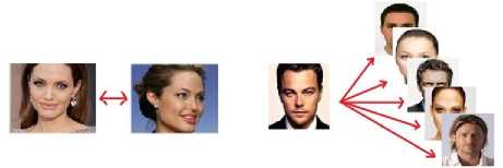
Image Face recognition among numerous applications of image processing plays a vital role in security and surveillance systems. In general, face recognition refers to either verifying or identifying a person from a digital image or a video frame. In case of verification, an unknown face image is compared with a known face image (Fig. 1-a) and for identification, a probe image is compared with a set of images (Fig. 1-b).
Nowadays face recognition is used in many devices and social media networks to make them more attractive and secure. This skill works well against changes in visual conditions such as facial expression, illumination, aging, make up and also occlusion by glasses, scarf, hats and beard or hairstyle. So far, many face recognition algorithms have been proposed [1-9]. In [1], singular value decomposition, 2D projections of principal component analysis (PCA) and linear discriminant analysis were studied. In [2], a technique called image matrix fisher discriminant analysis was introduced. In [3], PCA model was used to reduce the effects of illumination changes and facial expressions. In some methods, such as the local binary pattern (LBP) [4-5], texture was used as features. For instance, face recognition based on LBP features [6-8], and with Gabor wavelet filtering were proposed in [5], [9].
(a) (b)
Fig.1. Using face recognition for (a) verification, (b) identification.
In contrast with the conventional methods, sparse representation classification (SRC) [10-16] is new. The first implementation of SRC for face images was introduced in [10], which is robust to illumination changes and occlusion. A new frame work for non-upfront faces was proposed in [11]. Due to cropping, scaling or misalignment, the performance of two SRC mentioned methods would be degraded. In [12], authors tried to overcome the misalignment, occlusion and illumination variations by using the sparse representation. In [13], structured sparse representation was proposed for face recognition with occlusion. SRC was used for face recognition for multi view face images, which needs many poses for each subject to construct the gallery described in [14]. A pose robust method was presented in [15]. In [16], face recognition by using SRC on features extracted from faces proposed whereas unlike other SRC methods it doesn’t need alignment or canonical form of face and it works on holistic face or face patches with one sample for each subject.
Sparse representation is highly related to compressive sensing or compressive sampling (CS), a theory for sampling and recovering a signal from less samples than required by Shannon-Nyquist sampling theorem [17]. So, the CS based algorithms need lower sample rate in comparison with other methods. There are several recovery algorithms in CS, which each algorithm might be suitable for a specific application. In this paper, for face recognition, the performance of recovery algorithms are evaluated for two type of dictionaries (the corresponding methods named SRC and MKD-SRC) and under different scenarios. The considered recovery algorithms are matching pursuit [18] (MP), orthogonal matching pursuit [19] (OMP) and compressive sampling matching pursuit [19] (CoSaMP) as greedy algorithms and Homotopy [20].
In this paper, at first, we compare the face recognition accuracy by using SRC and MKD-SRC for three different standard face data base in order to choose the appropriate recovery algorithm. Then, the optimum values of four parameters for MKD-SRC implementation are obtained. We also suppose some changes to form the feature based dictionary for MKD-SRC and evaluate the achieved performance.
The rest of this paper is organized as follows, in Section 2 a brief review of CS theory and OMP recovery algorithm, PCA, LBP and local ternary pattern (LTP) are given. In Section 3 two face recognition algorithms named SRC and MKD-SRC are explained, where the SRC dictionary includes face images and the MKD-SRC dictionary includes the extracted features from faces. Experimental results presented in Section 4, and finally Section 5 contains the conclusion.
-
II. Background
In this Section, a brief review of CS and its recovery algorithms is presented, then PCA as a tool for dimension reduction and finally LBP and LTP as texture descriptors are explained.
-
A. CS Theory
Based on Shannon-Nyquist sampling principal [17], for perfect signal reconstruction, the sampling frequency must be at least twice the maximum frequency of interested signal. Therefore, in many applications like magnetic resonance imaging, there are great number of samples which make compression necessary before either storage or transmission. While sampling and compressing are performed in order, in CS they are done simultaneously.
Suppose w e RNx1 is a signal to be sensed (sampled), it can be expressed in ψ sparse domain, w = ^x (1)
where у e r N x N is the sparse matrix and x e R N x 1 is the equivalent representation of signal w in ψ domain. The signal w is s - sparse if it is combination of just ^ columns of ψ , or in other words x has only s nonzero coefficients, and the signal w is compressible if s << N .
Now, consider the measurement process,
У = Фw (2)
where y e R M x 1 is the observed vector, Ф e R M x N is the measurement or sensing matrix and M << N According to Eqs. (1)- (2), we have:
У = Ax (3)
where A = Φψ e R M x N named dictionary. The main challenges for CS applications [21] are 1) using a stable measurement matrix Φ such that the salient information in any s - sparse or compressible signal is not damaged by the dimensionality reduction from w e R N x 1 to y e R M x 1 2) finding a sparse domain where there is high incoherency between measurement and representation matrices and 3) using an algorithm to recover w from only M observed data y .
-
1) CS Recovery Algorithms
In general the CS recovery algorithms try to find a unique solution for under determined problem, Eq. (3), that means the number of unknown variables N are greater than the number of equations M . Different algorithms such as - 1 -norm [22-23] have been proposed where the main issues are sparsity of the solution and the algorithm time consuming.
x = argmin||x||i subjectto y = Ax (4)
x
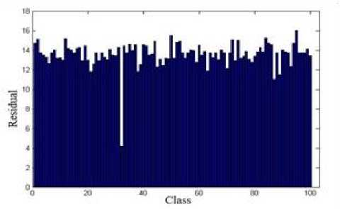
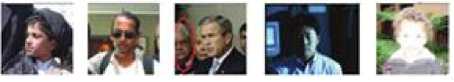
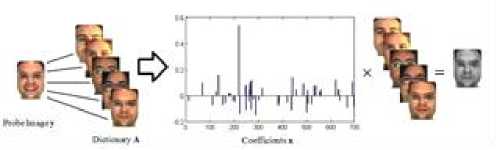
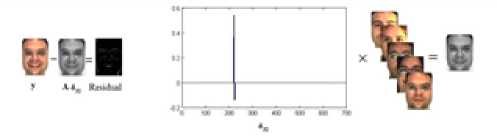
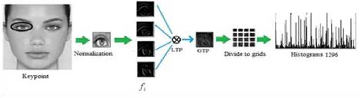
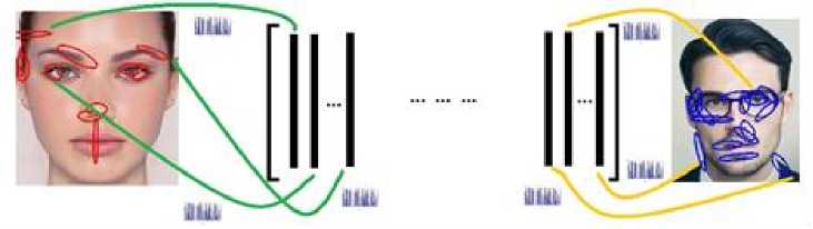
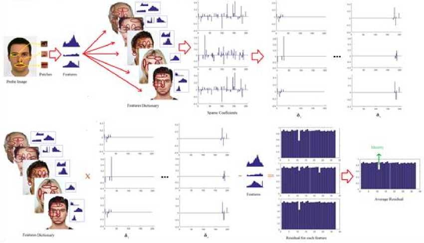
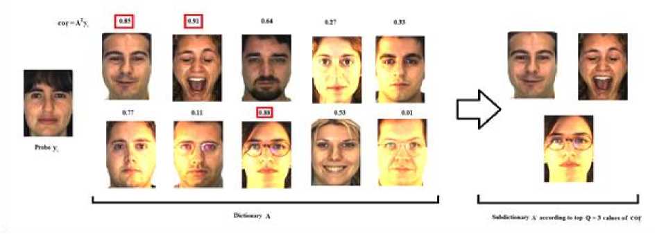
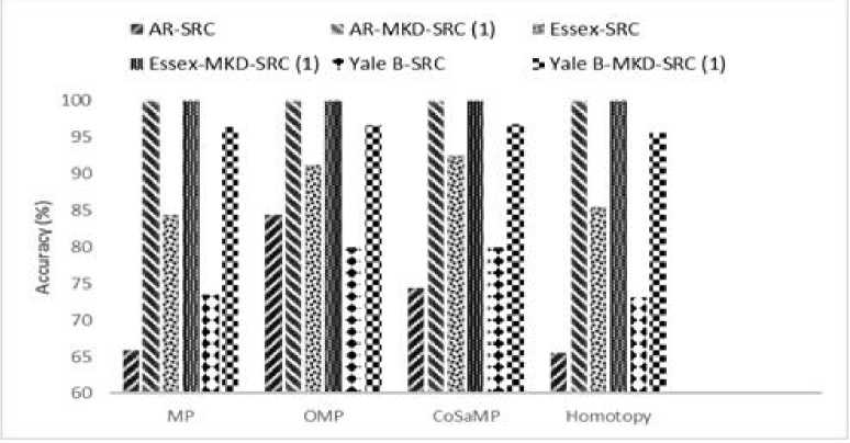
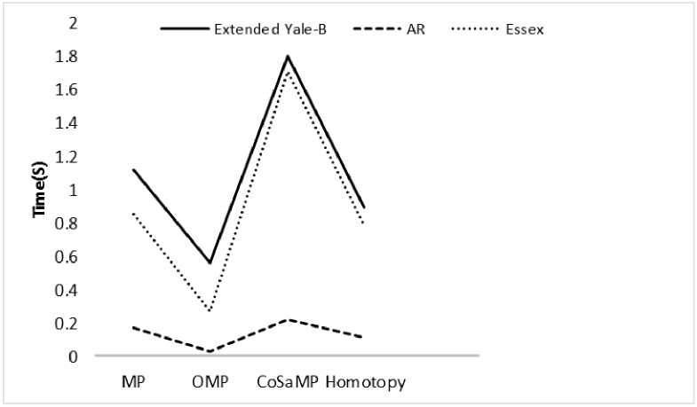
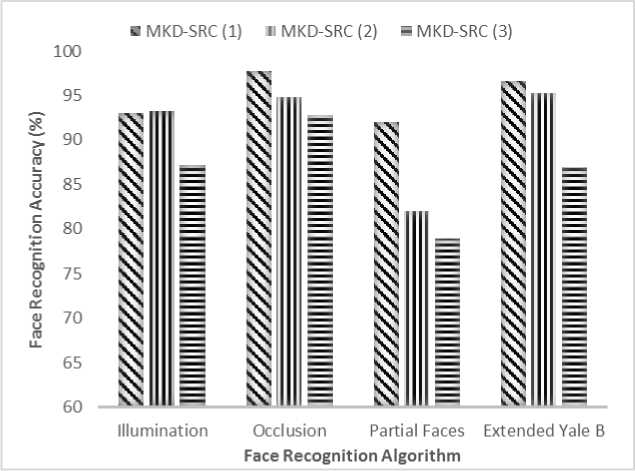
Eq. (4) can be rewritten by considering e as error, x = argmin||x||Z] subjectto ||y - Ax||^ x where in general for vector x = [Xi,X2,•••, xn] the Ip -N1 norm is (^| xj |p)p . Greedy algorithms [18-19], are i=1 well-known due to low complexity framework and fast run time. The core idea of greedy algorithms is finding the highest correlation between the residual of signal and the dictionary columns. In this paper, OMP as an efficient greedy algorithm, is explained in following to solve Eq. (4) or Eq. (5). For initializing, every atoms ( Ai e RMx1 ) of the dictionary A = [A1,A2,..., Ai ,...,AN ] e rMxN is normalized to have unit I2 norm, consider x0= 0 e RNx1 as initial solution, r0= y - Axo e RMx1as initial residual vector, and Λ 0 as a null matrix. Then, OMP runs the following steps for every iteration (j = 1,2,..., J), 1. Calculate the inner product g j[i] = Airj-1 e RMx1. 2. Find the index к where к = arg max | g [i]|. 3. Update the matrix of chosen atoms and related index set A. = A. UA , Л. = Л. , U{k} (the size of matrix 4. Evaluate ~ = (A^A л j)-1аЛ y as an estimation and update the coefficient vector x j[Л j ] = x (the size of x is growing with iteration number), where (.)T and (.)-1 are transpose and inverse operators. 5. Refresh the residual rj = y - Axj. 6. Repeat all steps until j is greater or || Гj |^ is less than the assumption values. i=1,..., N Л j Л j-1 К j j 1 Λ is growing with iteration number). pixel (xcenter, ycenter) , theneighbor pixel (xn, yn ) , the gray level g , and the windows size 9, the LBP is, LBP (x center, ycenter s(gn, gcenter) ) = 2 2ns(gn, g n=0 1 ifgn — gcenter 0 if gn > gcenter center) Although LBP features are robust to illumination changes, using the center pixel as the threshold value makes it sensitive to noise [4]. So in order to overcome this problem, LTP by using variable t was proposed [24], LTP(xcenter, ycenter) = 2 43 s(gn ’ gcenter, t) , n=0 1 if gn — gcenter + t s(gn, gcenter, t) 0 if| gn gcenter l< t — life <2 + — t ( A gn — gcenter L Fig. 2 shows the values of LBP and LTP for a sample center pixel. B. Principal Component Analysis PCA maps a set of data into linearly uncorrelated data and it is used for feature extraction and dimension reduction. Considering A = [A1, A2,..., Ai ,...,AN ] as an overcomplete or redundant dictionary with size M x N where M << N, the PCA procedures are, 1N 1. Compute the mean vector, g = 2 Ai . 2. Subtract the mean vector from all columns of Fig.2. Computing the LBP and LTP according to the s-function, Eqs.(6), (7). 3. Form the new centered dictionary, 4. Compute the covariance matrix, CMxM N =N 2 BiBT* i=1 5. Compute the eigen vectors {Vi }i=1:M and eigen values {Xi }i=1:M of covariance matrix C , where CVM= XVM , X1 > X2 > ... > XM . 6. Obtain U = {Vi }i=1:L corresponding to the L largest eigen values, where L << M << N and the reduced dictionary, ELxN = UTxM BMxN . i=1 dictionary, Bi = Ai - g . C. Local Binary Pattern (LBP) and Local Ternary Pattern (LTP) LBP [4] is a powerful texture descriptor that is robust to uniform changes in gray levels. Considering the center III. Face Recognition And Sparse Representation Although, automatically recognizing human faces from the facial images under different senarios has been an attractive research topics for many years, using the sparse signal representation is new for this subject. Now a days, application of sparse representation are widely spreading in many fields such as face recognition. Implementing the sparse representation needs using a proper reconstruction algorithm to recover the sparse signal and defining a dictionary as well. Although, OMP is a well-known and efficient greedy algorithm, defining the proper dictionary for specific application is still an open research. In this Section, two types of dictionaries based on input face images are investigated. The method whose dictionary is made by input face images directly called SRC, and the method whose dictionary is constructed according to the extracted features from the input face images named MKD-SRC. A. SRC Face Recognition A pioneer article used sparse representation for face recognition [10] was published in 2009 where the dictionary of each class is formed by, corresponding images stacked into columns of Ai = [pit ,pi2 ,...,pin ] e RMxn , and pi^ e RMx1is the nth image of i-th class. An unknown probe image y belongs to the i-th class can be represented as, У = Ai«i (8) where ai = [ai], ai2,..., ai ]Te Rnx1 . As the dictionary A = [A1, A2,..., Ai,..., AC ] e RMN ( M << N ) contains the whole training images of all C classes and N = nC , the matrix form of Eq. (8) is, У = Ax (9) where x = [0,...,0, ai , ai2,..., ain ,0,...,0]T with size N x1 . Ideally the nonzero coefficients of x should be related to just one class, and x is n-sparse. But in practice, the x elements might be related to multiple classes, though it is expected that the x elements belong to only one class. Therefore, as proposed in [10], the nonzero coefficients of x associated with the i-th class (i = 1,2,..., C) form the new vector named 6i(x) and then, the corresponding residual for every class is obtained as, ri (У) =||У — A8i(x)||22 (10) A class with minimum residual is the identity of probe image. This method is called SRC and the procedures for a probe sample image are shown in Fig. 3. (b) Fig.3. The SRC method for a sample probe is shown (a) obtaining the sparse coefficient vector xfor a sample probe belongs to AR dataset, (b) computing the residuals for every class based on Eq. (10), the probe belongs to that class with least residual [29]. B. MKD-SRC Face Fecognition In real world, face Images are taken under uncontrolled situations. In these scenarios, the images might include a partial faces which Fig. 4 showes some samples. Fig.4. Examples of partial faces [16]. Obviously SRC fails for partial faces, so, a method named multi key point descriptor-SRC (MKD-SRC) was proposed [16]. Briefly, for every images, MKD-SRC extracts patches [25], then feature vectors are obtained for the patches. The dictionary is consist of the feature vectors for the patches of all training images. The procedures of extracting a feature vector for a patch is shown in Fig. 5-a and listed in following. (a) 1. Use the Z-Score normalization to discard the illumination changes effect. 2. Consider the Gabor wavelet with one scale and four orientation 0°,45°,90°,135° (i = 0,1,2,3) and 3. Compute GTPi(x,y) = £3i[(fi(x,y) <-t) + 2(fi(x,y) > t)]. i=0 4. Divide the 40 × 40 resulting region into 4 × 4=16 cells, with size 10 × 10. 5. Compute the histogram of GTPs for every cell, and normalize by tanh(ax) to eliminate the outliers, where a is a constant, then form a 1296dimensional (4 × 4 × 81) feature vector. unique variance. Obtain the convolution of the patch with the imaginary part of Gabor kernel, the outputs named fi (X, y). Inspired by the LTP [24], considering t as threshold. The resulted descriptor named Gabor Ternary Pattern (GTP). As the highest value is 80 (2 x (33 + 32+ 31+ 30 ) = 80 ) and the lowest value is 0, so there are always 81 different GTPs. For every classes, the MKD descriptors including feature vectors are stacked into the matrix Ai = [di , di ,..., di ] e RMxik , and the gallery dictionary 1 2 ki including all the C classes is formed C A = [A 1}A2 ,...,Ai,...,Ac ]e RMxK , where K = ^ ki i=1 (see Fig. 5-b). Applying PCA for gallery dictionary to reduce the dictionary dimension to L , A e RLxK, where L << M . Being K >> L , in practice means that A is an overcomplete dictionary. Now for any probe image with k descriptors Y = [y^ „ym ,...,y k ]e RLxk (note that the length of every feature vector is reduced by using PCA.), the SR problem for every descriptor is, xm = argminixml|^ Subject tO ym = Axm, m = 1,2,..., k. (a) (b) (c) Fig.5. The MKD-SRC (1) method for a sample probe is shown (a) feature extraction, (b) dictionary construction, and (c) face recognition. For a given probe image, features are extracted and all features are compared separately with the dictionary which is built of features as well, to obtain all sparse coefficients, then sparse coefficients related to each class are obtained as δ (xˆ ) , then residual for each feature is computed using Eq. 12, finally a class with total least residual is the identity of probe image. Fig.6. For reduction the algorithm complexity, the sub dictionary with extremely few elements is constructed based on using Eq. (13). For better illustrations the face images are used instead of features. where xm e RKx1. In practice, the nonzero elements of xmmight be related to multiple classes, though it is expected that they belong to only one class. So, for face recognition based on MKD-SRC similar to SRC method, the nonzero coefficients of xmassociated with the i-th class (i = 1,2,..., C) form the new vector named Sc (xm ) and then the average corresponding residual for each class is obtained, k minrc(Y) = -£||yi -A6c(xi)|z (12) ck 2 i=1 A class with minimum residual is the identity of probe image. The algorithm explained above named MKD-SRC (1) does not need alignment, see Fig. 5-c. If in step 2 for Gabor Kernel, 8 orientations are used and also in step 3 LBP is used, the algorithm named MKD-SRC (2). And if in step 4, the number of cells are changed into 4, the algorithm named MKD-SRC (3). Since the dictionary A might have so many atoms, i.e. K is a large number, at every iteration of CS recovery algorithm, the number of inner products that should be computed is equal to K , it means the algorithm implementation is time consuming. In this paper, in order to overcome the mentioned problem, for every descriptor y, the linear correlation, cor e RKx1 is obtained as, ii cori = ATyi, (13) Next Corresponding to the Q ( Q << K ) greatest values of cori, the dictionary Ai e RLxQ is derived from A . Then, for Eqs. (11), (12) the dictionary A is replaced by Ai , see Fig. 6. IV. Experimental Results One major goal of this paper is to select a proper CS recovery algorithm for face recognition problem when two different type of dictionaries and different face datasets are used. For this purpose, three datasets called AR [26], Extended Yale-B [27], Essex University [28], are used. AR contains frontal face images of 126 people over 4000 images, with different illumination, expression and occlusion. We chose 100 subjects including 50 male and 50 female, there are 14 images for each person, captured at two sessions with varying illumination and expression [26]. In this experiment, for AR, the training set is consisted of 7 images of first session and for the test set, 7 images of second session are considered. Extended Yale-B contains frontal face images of 38 persons taken under different illumination conditions. We chose randomly half of 2414 total images for training set and remaining images as test set. Essex consists of 3040 frontal face images of 152 persons, captured in 20 consecutive frames. For every class we chose one image per individual as train and 19 images as test. The algorithms are implemented using Matlab on a PC with Core i7 CPU and 4GB of RAM. In general, MKD-SRC needs 4 parameters; i.e. ‘ L ’ for PCA, ‘ Q ’ for correlation, ‘ t ’ for threshold and ‘a’ for tanh. So finding the optimum values are a challenge for the algorithm implementation. In this paper for MKD-SRC (1), the optimum values are proposed according to the experimental results shown in Fig. 7. According to the achieved accuracy, as seen in Fig. 7, for AR, Extended Yale-B and Essex, the recommended range or value for parameters are L = 128 , t e [0.001 0.05] and a e [10 30]. Though Q = 10 has good performance we chose Q = 100 , since it has slightly better performance and the run time doesn’t have much difference. So, in following experiments and also for MKD-SRC (2) and MKD-SRC (3), we suppose L = 128 , Q = 100 , t = 0.03 , a = 20 . 100 ж ; < 70 64 128 256 512 L 100 ж 10 100 500 1000 Q -----AR — — Extended Yale В ...... Essex 100 л 0.001 0.01 0.03 0.05 0.07 0.1 g 90 ГО 80 3 и 3 70 1 10 20 30 No Fig.7. Finding the optimum values of reduction parameter " L " (top left), fast filtering parameter " Q " (top right), ternary pattern threshold " t " (bottom left) and tanh parameter "a" (bottom right) for MKD-SRC (1) according to the achieved accuracy. Regards to recommending a recovery algorithm according to the accuracy and computational cost where SRC and MKD-SRC (1) are used as face recognition approaches and AR, Essex, Yale-B are three different data set, as seen in Fig. 8-a, the achieved accuracy by using OMP and CoSaMP are nearly the same and greater than both MP and Homotopy. Therefore, considering the time consuming shown in Fig. 8-b, c, the OMP as the recovery algorithm is recommended as well. For evaluating three proposed MKD-SRC algorithms, three different scenarios on AR dataset using OMP recovery algorithm are supposed as 1) images with different illumination and expressions, 2) images with occlusion and 3) partial faces extracted and scaled from holistic faces. For all scenarios only one image per person (100 persons) is used as train and others as test, for instance, the first scenario (different illuminations), 7 images as test are used, the second scenario (occlusion), 12 images per person wearing sunglasses and scarf as test are used. The third scenario (partial), 100 images were chosen randomly and were cropped and scaled as test set. We also used Extended Yale-B dataset for this experiment. As Fig. 9 shows, MKD-SRC (1) is preferred for all scenarios except illumination variation where MKD-SRC (2) outperforms others. We also used kernel PCA (Gaussian and Polynomial Kernels) for dimension Reduction but it didn’t get an appropriate performance and therefore the results is not reported. (b) Е 400 AR Essex MP OMP CoSaMP Homotopy (c) Fig.8. Choosing the appropriate recovery algorithm for three datasets, AR, Essex, and Extended Yale-B, according to (a) face recognition accuracy, (b)-(c) algorithm run time in order for SRC and MKD-SRC (1). Fig.9. Face recognition accuracy for AR dataset with varying illumination, occlusion and partial faces and also for Extended Yale-B dataset. OMP as the recommended recovery algorithm is employed. V. Conclusion A dictionary plays an important role in face recognition based on sparse representation. In general MKD-SRC uses a dictionary built on extracted features and so in progress with partial faces. In this paper, we manipulated the procedure for constructing the dictionary and thereby introduce MKD-SRC (2) and MKD-SRC (3) in addition to the original MKD-SRC that named MKD-SRC (1). Furthermore, the performance of the proposed algorithms under employing four different recovery algorithms are compared and according to experimental results, CoSaMP and OMP are preferred but OMP is much faster than CoSaMP. Although the MKD-SRC have high accuracy, as it uses many features, the run time is so high compared to SRC though we try to overcome this problem by using the linear correlation. Based on our knowledge MKD-SRC wouldn’t have appropriate performance on face images with different poses as test set, when frontal face images are used as training set. Synthesis a frontal face image from different poses and then using MKD-SRC is the future research work.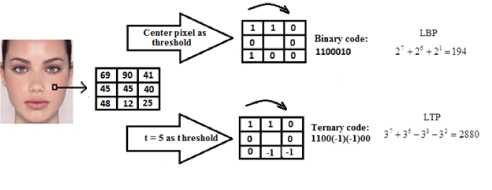
References Sparse representation and face recognition
- C. C. Chen, Y. S. Shieh and H. T. Chu, "Face image retrieval by projection-based features," in International Workshop on Image Media Quality and Applications, Kioto, 2008.
- C. Zhang, H. Chen, M. Chen and Z. Sun, "Image matrix fisher discriminant analysis (IMFDA)-2D matrix based face image retrieval algorithm," in International Conference on Advances in Web-Age Information Management, Hangzhou, 2005.
- H. C. Kim, D. Kim and S. Y. Bang, "Face retrieval using 1st-and 2nd-order PCA mixture model," in International Conference on Image Processing, New York, 2002.
- T. Ojala, M. Pietikäinen and D. Harwood, "A comparative study of texture measures with classification based on featured distributions," Pattern Recognition, vol. 29, pp. 51-59, 1996.
- T. Ahonen, A. Hadid, and M. Pietikainen, "Face description with local binary patterns: Application to face recognition," IEEE Transactions on Pattern Analysis and Machine Intelligence , vol. 28, pp. 2037-2041, 2006.
- T. Ahonen, A. Hadid, and M. Pietikäinen, "Face recognition with local binary patterns," in European Conference on Computer Vision, 2004.
- G. Zhang, X. Huang, S. Z. Li, Y Wang, and X. Wu, "Boosting local binary pattern (LBP)-based face recognition," in Advances in Biometric Person Authentication, 2004.
- S. Li, R. Chu, M. Ao, L. Zhang, and R. H, "Highly accurate and fast face recognition using near infrared images," in International Conference on Advances in Biometrics, 2006.
- W. Zhang, S. Shan, W. Gao, X. Chen, and H. Zhang, "Local gabor binary pattern histogram sequence (LGBPHS): A novel non-statistical model for face representation and recognition," in Tenth IEEE International Conference on Computer Vision (ICCV'05) , 2005.
- J. Wright, A. Yang, A. Ganesh, S. Sastry, "Robust face recognition via sparse representation," IEEE Transactions on Pattern Analysis and Machine Intelligence , vol. 31, no. 2, pp. 210-227, 2009.
- H. Li, P. Wang and C. Shen, "Robust face recognition via accurate face alignment and sparse representation," in International Conference on Digital Image Computing: Techniques and Applications (DICTA), 2010.
- A. Wagner, J. Wright, A. Ganesh, Z. Zhou, H. Mobahi and Y. Ma, "Toward a practical face recognition system: robust alignment and illumination by sparse representation," IEEE Transactions on Pattern Analysis and Machine Intelligence , vol. 34, no. 2, pp. 372-386, 2012.
- W. Ou, P. Zhanga, Y. Tanga and Z. Zhua, "Robust face recognition via occlusion dictionary learning," Pattern Recognition, vol. 47, no. 4, pp. 1559–1572, 2014.
- H. Zhang,, N. M. Nasrabadi, Y. Zhang, and T. S. Huang, "Joint dynamic sparse representation for multi-view face recognition," Pattern Recognition, vol. 45, no. 5, pp. 1292-1298, 2012.
- H. Zhang, Y.Zhang and T.S. Huang, "Pose-robust face recognition via sparse representation," Pattern Recognition, vol. 46, no. 5, pp. 1511-1521, 2013.
- S. Liao, A. K. Jain, and S. Z. Li, "Partial face recognition:alignment-free approach," IEEE Transactions on Pattern Analysis and Machine Intelligence, vol. 35, no. 5, pp. 1193-1205, 2013.
- P. Vaidyanathan, "Generalizations of sampling theorem; seven dacades after nyquist," IEEE Transactions on Circuits and Systems I: Fundamental Theory and Applications, vol. 48, no. 9, pp. 1094-1109, 2001.
- S Mallat, Z Zhang. , "Matching pursuit in a timefrequency dictionary," IEEE Transactions on Signal Processing, vol. 41, no. 12, pp. 3397-3415, 1993.
- L. Du, R. Wang, W. Wan, X. Yu, "Analysis on greedy reconstruction algorithms based on compressed sensing," in International Conference on Audio, Language and Image Processing (ICALIP), 2012.
- M. Asif, J. Romberg, "Sparse recovery of streaming signals using l1-Homotopy," IEEE Transactions on Signal Processing, vol. 62, no. 16, pp. 4209-4223, 2014.
- R. Baraniuk, "Compressive sensing," IEEE Signal Processing Magazine, 2007.
- E. Candes, J. Romberg, T. Tao, "Robust uncertainty principles: exact signal reconstruction from highly incomplete frequency information," IEEE Transactions on Information Theory, vol. 52, no. 2, pp. 489-509, 2006.
- D. Donoho, "Compressed sensing," IEEE Transactions on Information Theory, vol. 52, no. 4, pp. 1289-1306, 2006.
- X. Tan and B. Triggs, "Enhanced local texture feature sets for face recognition under difficult lighting conditions," IEEE Transactions on Image Processing, vol. 19, no. 6, pp. 1635-1650, 2007.
- "Scale & affine invariant feature detectors," 2012. [Online]. Available: http://www.robots.ox.ac.uk/vgg/research/affine/det_eval_files/extract_features2.tar.gz.
- M. Martinez, "The Ohio State University," 24 Jun 1998. [Online]. Available: http://www2.ece.ohio-state.edu/~aleix/ARdatabase.html.
- Kuang-Chih Lee, Jeffrey Ho, and David Kriegman, "The extended Yale face database B," [Online] http://vision.ucsd.edu/~leekc/ExtYaleDatabase/ExtYaleB.html.
- L. Spacek, "University of Essex," 20 Jun 2008 . [Online]. Available: http://cswww.essex.ac.uk/mv/allfaces/.
- S. Ghofrani, R. Alikiaamiri, M. Khorasani, "Comparing the performance of recovery algorithms for robust face recognition," in CGVCVIP 2015 Proceedings, 2015.
