Spatiotemporal Data Fusion using Dictionary Learning and Temporal Edge Primitives

Space borne global sensors observe synoptically the dynamic changes on the Earth’s surface at predefined intervals. This observed data plays a key role to understand the global water, carbon, and nitrogen cycles [10]. The structural information of the Earth’s surface can be obtained from the high spatial resolution sensor and its temporal variability can be obtained from the high temporal resolution sensor. But, there is a trade-off between high spatial and high temporal resolutions in designing space borne global sensors. For example, high spatial resolution sensors usually result in a smaller swath width, so that the revisit time is increased to view the same location on the Earth [5]. Conversely, high temporal resolution sensors have a more frequent revisit rate and produce larger swath width with a lower spatial resolution ([11]; [17]). These factors limit the applications that require the data in both high spatial and high temporal resolutions. Another possible way to meet the requirement is to merge the data from sensors with different spatial and temporal resolutions.

The ISRO Resourcesat-2 mission aims for the natural resources mapping and monitoring of the Earth’s surface [17]. The Resourcesat-2 LISS III sensor’s data have proven utility for land cover type changes [19]. Its 24-day temporal resolution is a long period for monitoring the bio dynamics of the Earth’s surface features and may create difficulties in mapping vegetation conditions in a timely manner. The spatial resolution of LISS III sensor is 23.5 m and the temporal resolution of AWiFS sensor is 5 days. This paper presents a novel fusion method to merge the LISS III sensor data with AWiFS sensor data to create a synthetic LISS III image at 23.5 m spatial and 5-day temporal resolutions.

Recently, the spatiotemporal data fusion methods are developed through single-image super resolution techniques. These techniques are implemented with the dictionary learning and the sparse representation methods (Hunag and Song.2012; [21]). The sparse representation methods use low spatial resolution (LR) and high spatial resolution (HR) image patches to derive low and high resolution dictionaries. Each patch in an image can be represented as a linear combination of atoms in a dictionary and the corresponding sparse coefficients [26]. Assume that the dictionary which describes the image patches as a periodic table of the fundamental elements (atoms) in the Chemistry. The combination of atoms forms a molecule, in a similar manner the linear combination of atoms in a dictionary and the sparse coefficients forms an image patch [7].

Yang et al (2010) [23] proposed a single image super resolution based on the sparse representation. This method jointly trains two dictionaries for high frequency details of LR and HR images, and these dictionaries are used to enforce the similarity of sparse representations between the low and high resolution patch pair. Compared to the Freeman et.al (2002) [9] approach, the learned dictionary pair is more compact representation of image patch pairs and it produces more competitive results.

The “Sparse representation-based Spatio-Temporal reflectance Fusion Model” (SPSTFM) developed by Huang and Song (2012) [12]. It is based on the singleimage-super resolution though dictionary learning. The HR and LR dictionaries are jointly trained with the image patches of HR and LR images. With these two dictionaries, it establishes a relationship between the structures within the HR images and their corresponding LR images. This model requires two MODIS (500 m)-Landsat (30 m) image pairs at time 1₁ and t₃ to predict a synthetic Landsat image for the MODIS image at time t₂ (t₁< t₂< t₃) . Whereas single-image-super resolution uses numerous LR-HR image pairs for a prior knowledge for the desired HR image.

Due to cloud coverage and low revisit rate, the two Landsat images may not be available. Moreover, it is very time consuming to identify these two Landsat images for a particular observation period (t₁ < t₂<  t₃) . To overcome this difficulty, the Song and Huang (2013) [21] developed a spatiotemporal data fusion method with only one MODIS-Landsat image pair. This fusion is achieved in two stages. In the first stage, transition images are obtained for the time and . The transition images are derived from the LR and HR dictionaries. The LR dictionary is trained with the gradient feature image patches of MODIS image and the HR dictionary is obtained by forming a minimization problem with high frequency image patches of Landsat image and the same sparse coefficients which are obtained in the LR dictionary training. In second stage, the high frequency details which are obtained from the difference image of Landsat image and the transition image of time are proportionally injected into the transition image of time

. Therefore the synthetic Landsat image for the time is obtained with the MODIS image at time and a single MODIS-Landsat image pair at time .

Spatiotemporal data fusion makes it possible to generate synthetic images at high spatial and high temporal resolutions. In synthesis of multi-sensor and multi-temporal data, spurious spatial discontinuities are inevitable [13]. The aforementioned methods have not dealt with these spurious spatial discontinuities. We propose a novel approach to minimize these spurious spatial discontinuities in the spatiotemporal data fusion.

Objective of the paper is to create a synthetic LISS III image for the time from an AWiFS image at time and a single AWiFS-LISS III image pair at time t0, where t0 * tk. The LR dictionary was trained with the gradient feature image patches of an AWiFS image for time  t0  using K-SVD algorithm [1], and the corresponding HR dictionary was derived by formulation of minimization problem with the high frequency image patches of LISS III image at time and the same sparse coefficients which were derived in the LR dictionary training. The two transition images were derived using these LR and HR dictionaries and an orthogonal-matching-pursuit (OMP) sparse coding technique [6]. Then, the high frequency details which were obtained in the difference of LISS III image and the transition image at time t0 were proportionally injected into the transition image at the time . The resultant image contains spurious spatial discontinuities. These discontinuities were identified with the temporal edge primitives and smoothed with the spatial-profile-averaging method.

• II.    R elated study

• A.    Sparse representation and dictionary learning

If values of a vector x are most of them close to zero, that vector is said to be a sparse. A signal is not sparse, we can make it sparse by transforming into another domain, for example, if x is sine, clearly it is not sparse. But Fourier transform of x is sparse [22].

A signal x can be written as a linear combination of T elementary waveforms (signal atoms), such that x = D a)                  (1)

Where a = [x ,, x ₂,..., x_M]^T and a = [ a ₁, a ₂,..., a_N]^T, a, are called the sparse representation coefficients of x in the dictionary D = [d ,, d ₂, ...,d_M]. Suppose the size of the signal x is N x 1, size of a is M x 1 and the size of the dictionary D is N x M and whose columns d y are the atoms, in general normalized to a unit Z₂ norm, i.e. for all j = 1,2..... m, ydyJI^Z 'LJ dyl ² =1.

The dictionary D = [d_x ,d₂, ...,d_r] is an indexed collection of atoms dj. The interpretation of d y depends upon the dictionary. For example, frequency for the Fourier dictionary (i.e. sinusoids), Kronecker basis (standard unit vectors) for the Dirac dictionary, positionscale for the wavelet dictionary, translation-duration-frequency for cosine packets, and position-scale-orientation for the curvelet dictionary in two dimensions [22]. All these dictionaries are fixed dictionaries to their corresponding mathematical transforms. The sparse representation provides further sparsity by learning the over complete dictionaries directly on the data. An over complete dictionaries are occurred if the number of coefficients are larger than the number of signal samples (i.e. M >  N ). This redundancy is avoided in data compression applications. But in image restoration applications this redundancy had proven the advantage to have fast analysis and synthesis [22]. The aforementioned sparse representation formulation in Equation (1) is for a single vector x. Now, the following paragraphs describe the dictionary learning procedure for the image patches.

Mathematical transforms may not always represent all the contained features in an image, because they are based on the fixed dictionaries. Sparse representation methods facilitate to learn the dictionary adaptively from the local structures within the image [20]. Each image patch x, of size Vn x Vn is lexicographically ordered and stacked into a matrix X = [xx ,x2, ,„,xw], where each is a column vector of size x 1 and hence the size of the matrix is x . To find the best dictionary to represent a given training samples , we have to solve the following optimization problem.

min , ‖ X - DS ‖ 2 subject to ‖ Si ‖ q ≤ k_Q for all I .

Where D =[di, ^2 ,…, d_M ] and S =[Si, S2,…,S/y], each d_z is of size n×1 and hence the size of D is n × M , each s_t is of size M ×1 and hence the size of s is M × N . The term ‖ s_t ‖Q means that the number of non zero terms in the sparse column vector s, is fixed and predetermined number of coefficients /(q . The above optimization problem can be solved with K-Singular Value Decomposition (K-SVD) algorithm [1]. The K-SVD algorithm is an iterative process to identify the best dictionary and sparse coefficients matrix. It updates an atom in the dictionary and the corresponding sparse coefficients at the same time. This simultaneous updating is speed up the convergence of the training process [7]. More details about the K-SVD can be found in Aharon et al. (2006) [1].

We found the dictionary D and the corresponding sparse coefficients matrix S for a given training samples X using the K-SVD algorithm. Now, we can find the sparse coefficients for a specific patch X (lexicographically ordered) with respect to the trained dictionary D in Equation (2) by using following approximation formula.

̂= arg min‖ s ‖ о subject to ‖ x - Ds ‖2≤ E (3)

Here £ is the error tolerance. The above sparse approximation problem can be solved with the sparse coding technique such as Orthogonal-Matching-Pursuit (OMP) [6]. The OMP start initially with s^k = , it iteratively constructs a к -term aproximant s^k by keeping set of active columns in the dictionary D at each stage. More details about the active columns selection is described in Elad. (2010) [7].The chosen active columns reduces the error ‖ x - Ds ‖2 at each stage, if it falls below the specified error threshold £ , the process terminates.

• B.    Single-image-super resolution through dictionary learning

  The single-image-super resolution techniques enhance the spatial resolution of a single low spatial resolution image. The single-image-super resolution ([2], [9], [4], [7]), first proposed by and Kanade (2000) [2], attempts to capture prior correspondence between LR-HR image patches. This correspondence is derived from the numerous LR-HR image pairs and applies this correspondence to predict an HR image from a LR image. Jiji et al. (2004) [15] proposed the wavelet transformbased single-image super resolution. The wavelet coefficients are learned from a set of LR-HR training image pairs at finer scales for the desired high resolution image. The learned image further regularizes with smoothness prior while super-resolving a given low resolution image. Wu et al. (2011) [25] proposed contourlet transform based single-image super resolution. A low-resolution (LR) image is decomposed sub bands with the contourlet transform. The unknown high-

• frequency coefficients for the input low-resolution image are inferred by a belief propagation algorithm. These high-frequencies are obtained from the Markov Random Fields (MRF) model together with the contourlet coefficients of numerous LR-HR image pairs in the training data.

The wavelet and contourelet transforms are based on the fixed dictionaries. In recent times, single -image-super resolution methods use adaptive dictionaries which are learned from the local structures within an image. Yang et al (2010) [23] first proposed a super resolution method based on the dictionary learning and the sparse representation. The low and high resolution dictionaries are jointly trained from the low and high resolution image patches. It enforces the similarity of sparse representations between the low and high resolution image patch pairs with respect to their LR and HR dictionaries. Hence, the linear combination of the sparse coefficients of a given low resolution image patch and the atoms in high resolution dictionary produces a high resolution image patch.

Zeyde et al. (2012) [26] improves the Yang’s algorithm in terms of the computational complexity and the algorithm architecture. Instead of training both low and high resolution dictionaries, Zyede’s method trained only low resolution dictionary using K-SVD algorithm. The high resolution dictionary is derived by formulation of minimization problem with the high frequency image patches of high resolution image and the sparse coefficients matrix which is derived in the low resolution dictionary training. The sparse-land models on the image patches works as regularization term or prior information in both Yang et al (2010) [23] and Zeyde et al. (2012) [26] methods. The aforementioned methods use numerous LR-HR image pairs for the dictionary training. But our spatiotemporal fusion method used only one LR-HR image pair. The multi-temporal images of the same geographic area have the high structural similarity between two consecutive dates so that we have used only one LR-HR image pair. In this paper, we used K-SVD algorithm to train the dictionary for the low and high resolution image patches. The sparse representation of a given image patch was obtained with the sparse coding technique OMP.

• III.    P roposed M ethodology

  The aim of the study is to create a synthetic LISS III image at time ^k with an AWiFS image at time ^k and a single AWiFS–LISS III image pair at time ^0 , here ^0 ≠ tk . Such synthetic LISS III image can be created through a spatiotemporal data fusion technique. Recently, Song and Hunag (2013) [21] developed a spatiotemporal data fusion based on the single-image-super resolution technique. This method uses a single MODIS-Landsat image pair as a prior knowledge. Originally, Song and Huang (2013) [21] method is two layer framework, each layer consists of two stages, the first is a super resolution stage and the second is a high pass modulation stage. Since the spatial resolution ratio of AWiFS and LISS III

  images are very small when compared to that of MODIS and Landsat images, the proposed method was adopted only one layer framework of the Song and Huang (2013) method [21]. In composition multi-sensor and multitemporal images, spurious spatial discontinuities are inevitable. The Song and Huang (2013) [21] method have not deal with these spurious spatial discontinuities. Moreover, this method enhances the spatial resolution of low resolution image with super resolution technique and then high pass modulation technique. But both superresolution and the high-pass-modulation techniques improve the spatial resolution. Their sequential implementation over enhance the spurious spatial discontinuities in the synthetic images. In this paper, we propose a novel approach to identify these spurious spatial discontinuities through temporal edge primitives. These discontinuities were smoothed with the spatial profile averaging method.

• A.    Super resolution of low spatial resolution image

The ideal parameters in consideration to fuse the data from different sensors are identical spectral bands, similar solar geometry, similar orbital parameters and the same time of acquisition [24]. The ISRO Resourcesat missions make it possible to acquire AWiFS, LISS III data simultaneously at identical spectral bandwidths, different spatial and radiometric resolutions at various swaths. Hence, AWIFS and LISS images met the most of the ideal conditions due to the acquisition from the same platform. Although AWiFS and LISS III sensors have similar spectral bandwidths, surface reflectance values of AWiFS were normalized to the reflectance of LISS III by the linear relationship between the homogeneous regions of AWiFS image and their corresponding regions of LISS III image [3].

In this section, the spatial resolution of AWiFS image was improved by the dictionary learning. The improved AWiFS images were called as the “transition images” as in Song and Huang (2013) method [21]. Denote AWiFS, LISS III and the transition images at time t0 as A0, L 0 and T0, respectively. The super resolution of low spatial AWiFS image contains two steps: The low and high resolution dictionary training and the transition image prediction. For low resolution dictionary training, extract the 5x5 patches from the gradient feature space of A0. These patches were rearranged into columns and these columns were stacked into a training sample matrix X . For high resolution dictionary, extract the 5×5 patches from the difference image L 0 — A0. These patches were also rearranged into columns and these columns were stacked into a training sample matrix Y. The columns of and are in one-to-one correspondence. The low resolution dictionary      is derived with following optimization problem

{D _z * ,S * } = arg min||X — D _г5Н г   sub; ec to

Di ,S

Ils JIg ^ ^ 0 for al I i.                (4)

Where D * ,S* was computed with the K-SVD algorithm. And S* is the sparse coefficients matrix for the training samples X with respect to the dictionary D*. To establish a relationship between low and high resolution dictionary, the same sparse coefficients matrix * was used to derive the high resolution dictionary. The high resolution dictionary      was constructed by minimizing the error on Y with the same sparse coefficients matrix *

D * * = a rg min   d *IIY — D _ftS * H ^ )       (5)

The Equation (5) can be solved directly with pseudo inverse (here ^* is a full rank matrix)

D * = Y(S * ) ⁺ = YS *^r (S * S *^r ) "¹         (6)

Now, we have both low and high resolution dictionaries    and . The transition image    was derived from A0 , extract the 5x5 patches from the gradient feature space of , rearranged into columns, and these columns were stacked into a matrix X0. Denote the columns of    as     and its sparse coefficients column with respect to the dictionary was obtained with the sparse coding technique OMP. This sparse coefficients column     was used to obtain the corresponding high resolution patch. Since the low and high resolution training samples are enforced to represent the same set of sparse coefficients columns, the corresponding high resolution patch column can be predicted with у0, = D* * s,. After rearranging all the columns      into patches, we obtained a difference image Y0 between T0 and A0 , and hence T0 = Y0 + A .In a similar manner, the transition image was predicted for the time .

• B.    Spatiotemporal data fusion via high pass modulation

The training image pair AWiFS A₀ - LISS III L ₀ at time has many similarities with the image pair AWiFS

• - LISS III    at time in regard to crop phenology

  and land-cover-type changes in most of the time except sudden land-cover-type changes. The predicted transition images and are almost similar to the LISS III images. As in Song and Huang (2013) [21] method, we assume that the pixel purity is same between (   )

and (  ) and there is a linear relationship between and in temporal changes. Then

T_k (i, j) = aT( (i ,j) + b             (7)

Where ( , ) is a given pixel location and and are linear regression coefficients for relative temporal change from the time to . Since the pixel purity is same between (   ) and (  ), it is reasonable to assume that the linear relationship between and    .

L_k ( I, j ) = aL о ( I, j) + b              (8)

From Equation (7) and Equation (8), we obtain

Lk(i, j) = Tk (i,j) + a[L0 (i,j) - TQ (i,j) ]    (9)

The scalar value a can be approximated as T_k ( i, j )/ To (i , D . Then Equation (9) is written as

L_k = T_k + №) [L_o - T_o ]        (10)

Equation (10) shows that the  high  frequency information of time proportionally transfers to the time by using high pass modulation, which is also widely used in pan sharpening. Since Lo, To and Tk are already known, we can predict synthetic LISS III image for the time .

• C.    Smoothing the spurious spatial discontinuities

  In this paper, section 3.1 and 3.2 describe the first and the second phase of the proposed method, which are similar to the one layer framework of the Song and Huang (2013) method [21]. In third phase, we propose a novel approach to identifying and smoothing the spurious spatial discontinuities which are occurred in the spatiotemporal data fusion of multi-sensor and multitemporal images. In the third phase, there are two stages. In the first stage, spurious spatial discontinuities were identified with the temporal edge primitives. In the second stage, these spurious discontinuities were smoothed with spatial-profile-averaging method.

C.1. Stage 1: Temporal edge primitives

The human visual system is more sensitive to sharp contrast changes than the smooth regions in an image (Ji et al.1994). Sharp contrast changes form image primitives such as contours, edges or ridges. In temporal data composition, spurious spatial discontinuities are inevitable for land-cover-type changes [13]. The reason for these spurious spatial discontinuities is the pixels around the changed feature are originated from images with different days with different sun-pixel-sensor viewing geometries. We identified these spurious spatial discontinuities using temporal edge primitives which were extracted with the following steps.

(a)

(b)

(c)

High frequency details were extracted from AWiFS images at the time t0 and tk using 3x3 Laplacian

— 1  —1—1

high-pass filter (—1   8—1

—1 —1—1

points, lines and edges in the image and suppresses

uniform and smoothly varying regions.

From these high frequency details, edges are detected with Canny edge detection method. These edges were called as temporal edge primitives at the time and .

Subtract the edges at the time from the edges at the time .

If edges are in the same location at the time t0 and tk , both the edges are cancelled. If edges are in different location at the time and , both the edges are retained. Black color edges represent the edge pixels at the time t0

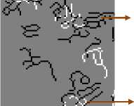
(a)

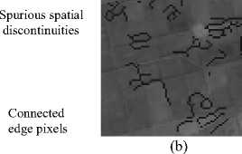
Fig.1. Indentifying the Spurious Spatial Discontinuities using Temporal Edge Primitives (a) Temporal Edge Primitives (b) Spurious Spatial Discontinuities in Stage 1

in Fig.1 (a). White color edges represent the edge pixels at the time tk in Fig.1 (a). Due to sub-pixel level geometric bias between the two AWiFS images at the time and , same edge may represent in both black and white as connected edge pixels side by side as shown in Fig.1 (a).

The edge pixels which are cancelled, white color edge pixels and connected edge pixels are important to retain the spatial discontinuities for the time tk. After ignoring all these edge pixels, only black color edge pixels are identified as spurious spatial discontinuities and they are overlaid on the predicted image in section 3.2 as shown in Fig.1 (b). The surrounding pixels of these black color edge pixels will have spurious pixel values which were occurred due to land-cover -type changes from the time to . These spurious spatial discontinuities are smoothed by the spatial profile averaging between the homogeneous pixels of AWiFS image at the time tk and the pixels around the black colour edges in the predicted image in section 3.2.

C.2. Stage2: Spatial profile averaging

Consider a 7x7 window around the black colour edge pixels as 2-dimensional spatial profiles in the predicted image in section 3.2. At the same location, consider the pixel values in a 7 x 7 window of the AWiFS image at the time tk as 2-dimensional spatial profiles.These 2dimensional profiles represent the shape of the surface. Shape-based averaging preserves the contiguous regions of an image [18]. Average of these two 2-dimensional spatial profiles smoothed the spurious spatial discontinuities in the predicted images.

It highlights

(a)                       (b)                        (c)

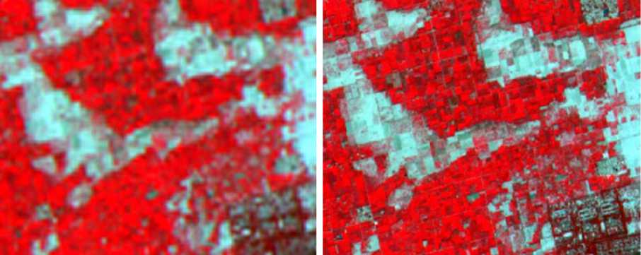
Fig.2. Smoothing Spurious Spatial Discontinuities Using Spatial Profile Averaging (a) Predicted Image after Super Resolution and High Pass Modulation Phases (b) Predicted Image after Super Resolution, High Pass Modulation and Third Phase (c) Original LISS III Image

The resultant image is shown in Fig.2 (b) which is almost similar to the original image in Fig.2(c). If the size of the window increased, spatial profile averaging over smoothed the image. Fig 3 shows the flowchart of the proposed method.

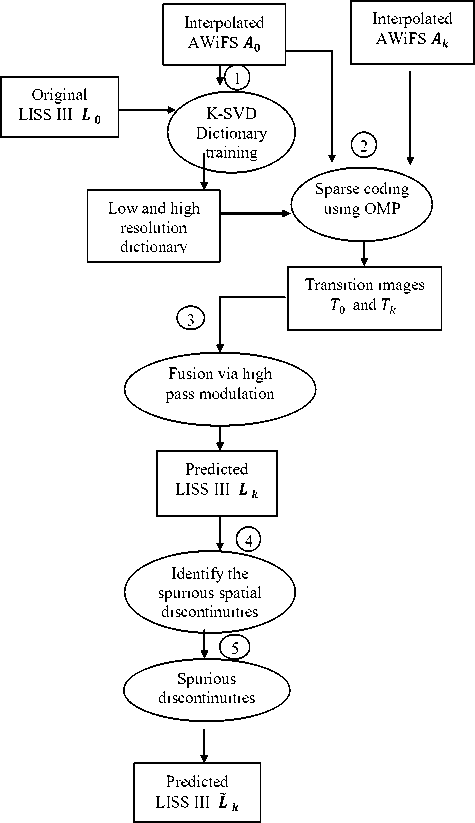
Fig.3. Flow Chart of the Proposed Spatiotemporal Data Fusion Using Dictionary Learning and Temporal Edge Primitives

• IV.    E xperimental R esults A nd C omparisons

  In this section, the proposed method is compared with the recently developed Song and Huang (2013) method (SH method) [21]. Experiments are conducted with AWIFS and LISS III datasets. In pre-processing, AWiFS and LISS III image pixel values were converted into Top-Of-Atmosphere (TOA) reflectance. Further, reflectance values of AWiFS were normalized to the reflectance of LISS III by the linear regression between the homogeneous regions of AWiFS image and their corresponding regions of LISS III image with the procedure described by the [3].

• A.    Experimental data set: 1 with focus on crop phenology changes

  In this experiment, we have used previously acquired single AWiFS-LISS III image pair and a single AWiFS image to predict a synthetic LISS III image at AWiFS temporal resolution. For experimental demonstration of the proposed method, 12 km × 12 km area was selected in the Suratgarh area in Rajasthan state of India to predict the crop phenology at LISS III spatial and an AWiFS temporal resolutions. Single AWiFS–LISS III image pair acquired on 24-Sept-2012 was used as prior knowledge to predict a synthetic LISS III image for 18-Oct-2012 by using an AWiFS image acquired on 18-Oct-2012. These data sets show more crop phenology change from 24-sept-2012 to 18-Oct-2012 than the land-cover type changes as shown in Fig. 4.

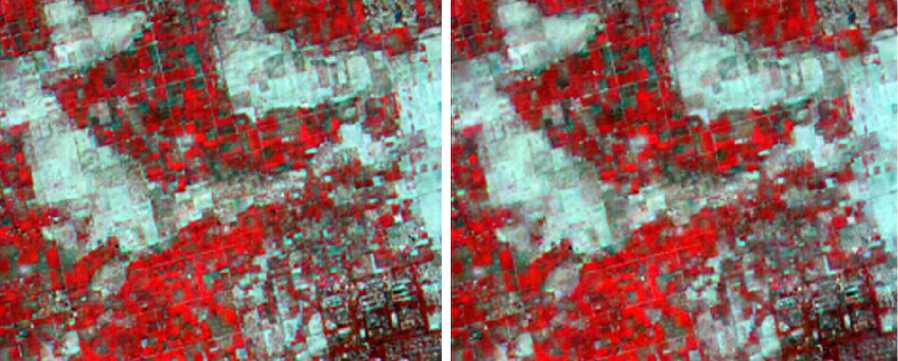
The proposed method is compared with SH method with DL of dictionary size: 1000. Number of iterations is 30 for K-SVD and the size of the images is 512×512. Fig 4(e) shows the predicted synthetic LISS III image by using SH method and Fig 4(f) shows the predicted synthetic LISS III image by using the proposed method. Fig 4(f) more resembles than the Fig 4(e) to the original image in Fig 4(d).

The comparison of the four bands (Green-Red-NIR-SWIR) between SH method and the proposed method in terms root means squared error (RMSE), structural similarity index map (SSIM), and spectral angle mapper (SAM) is described in Table 1. The average RMSE of four bands for SH method is 0.0111 and for our method is 0.0100, it shows that the proposed method has better image quality when compared to the SH method. The average SSIM of four bands for SH method is 0.9074 and for our method is 0.9288, it shows that the proposed method shows high structural similarity with the original image than the SH method. Also, the proposed method has less spectral distortion than SH method with reference to the SAM values shown in Table 1.

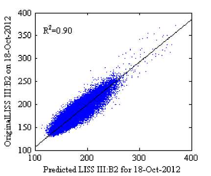
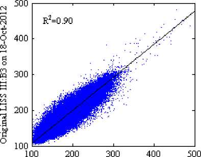
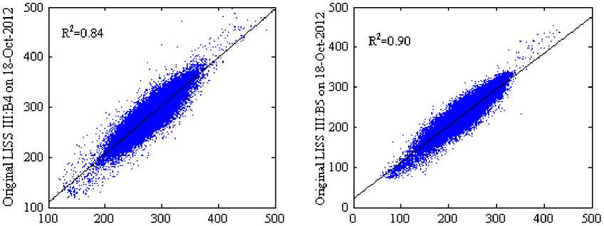
The scatter plots with R² in Fig 5 and 6 (where the scale factor is 1000) show the reflectance distribution between the predicted and the actual surface reflectance of the four bands, Fig 5(a)-5(d) scatter plots of the predicted surface reflectance by using SH method and Fig. 6(a)-6(d) scatter plots of the predicted surface reflectance by using our method against the actual reflectance. The average R² of four bands for the SH method is 0.8575 and for the proposed method is 0.8850, it indicates that our method predicts reflectance values more accurately than SH method. Visually, it can be observed that the result of the proposed method in Fig 4(f) shows a similar perception as in original image Fig 4(d) when compared to the SH method.

a. aw i fs on 24-s ept - 2012                                    b^. LISS III ^on 24^-S^ept^-2012

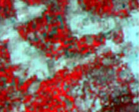
(c). AWiFS on 18-Oct-2012

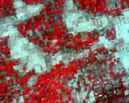
(d). Original LISS III on 18-Oct-2012

(f). Predicted LISS III for 18-Oct-2012 using proposed method

(e). Predicted LISS III for 18-Oct-2012 using Song and Huang (2013) method

Fig.4. Predicted LISS III Images in Green-Red-NIR False Color Composition using (e) Song and Huang (2013) method and the (f) Proposed Method with the Prior Knowledge (a), (b) and (c).

Table 1. Quantitative Comparison of the Proposed Method against SH Method for the Dataset: 1

Method	SSIM				RMSE				SAM
	B2	B3	B4	B5	B2	B3	B4	B5
Proposed method	0.9434	0.9269	0.9175	0.9275	0.0071	0.0130	0.0100	0.0102	1.8523
Song and Huang (2013)	0.9262	0.9011	0.8916	0.9108	0.0082	0.0143	0.0114	0.0107	2.1309

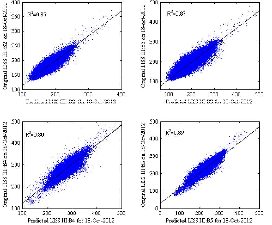
Predicted LISS III :B2 for 18-Oct-2012

Predicted LISS IILB3 for 18-Oct-2012

Fig.5. Scatterplots of the Predicted Against the Actual Surface Reflectance for the Song and Huang (2013) Method

Predicted LISS IILB3 for 18-Oct-2012

Predicted LISS IILB4 for 18-Oct-2012

Predicted LISS IILB5 for 18-Oct-2012

Fig.6. Scatter Plots of the Predicted Against the Actual Surface Reflectance for the Proposed Method

• B.    Experimental data set: 2 with focus on rapid landcover-type changes

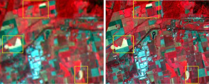
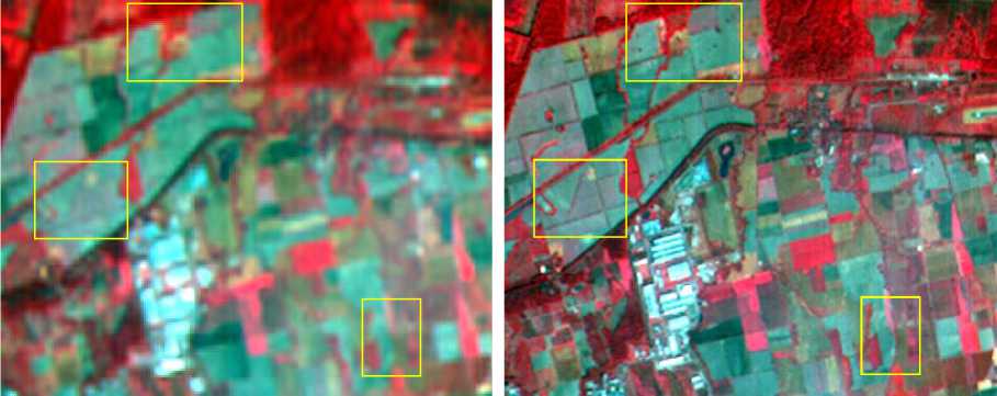
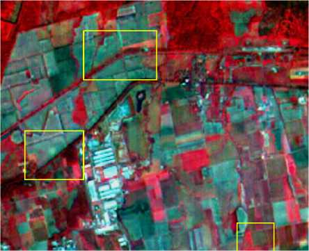
  In this experiment, 12 km x 12 km area was selected in Pantnagar area in Uttaranchal state of India to predict the land-cover-type changes at LISS III spatial and AWiFS temporal resolution. Single AWiFS -LISS III image pair acquired on 24-Oct-2012 was used as prior knowledge to predict a synthetic LISS III image for 17-Nov-2012 by using the AWiFS image acquired on 17-Nov-2012. This data set has both crop phenology changes and land cover type changes such as bare soil on 24-Oct-2012 converted into wet land on 17-Nov-2012 as shown in Fig 7. These land cover type changes are shown in yellow colour boxes in Fig 7.

The proposed method was compared with SH method with DL of dictionary size: 1000. Number of iterations is 30 for K-SVD and the size of the images is 512x512. Fig 7(e) shows the predicted synthetic LISS III image by using SH method and Fig 7(f) shows the predicted synthetic LISS III image by using the proposed method. Fig 7(f) more resembles to the original image in Fig 7(d) than the Fig 7(e).

The comparison of the four bands (Green-Red-NIR-SWIR) between SH method and the proposed method in terms root means squared error (RMSE), structural similarity index map (SSIM), and spectral angle mapper (SAM) is described in Table 2. The average RMSE of four bands for SH method is 0.0130 and for our method is 0.0117, it shows that the proposed method has better image quality when compared to the SH method. The average SSIM of four bands for SH method is 0.8668 and for our method is 0.8966, it shows that the proposed method shows high structural similarity with the original image than the SH method. Also, the proposed method has less spectral distortion than SH method with reference to the SAM values shown in Table

The scatter plots with R² in Fig 8 and 9 (where the scale factor is 1000) show the reflectance distribution between the predicted and the actual surface reflectance of the four bands, Fig 8(a)-8(d) scatter plots of the predicted surface reflectance by using SH method and Fig 9(a)-9(d) scatter plots of the predicted surface reflectance by using our method against the actual reflectance. The average R ² of four bands for the SH method is 0.7375 and for the proposed method is 0.7850, it indicates that our method predicts reflectance values more accurately than SH method. Visually, it can be observed that the result of the proposed method in Fig 7(f) shows a similar perception as in original image Fig 7(d) when compared to the SH method.

a. AWiFS on 24-Oct-2012                                 (b). LISS III on 24-OCT-2012

(c). AWiFS on 17-Nov-2012

(e). Predicted LISS III for 17-Nov-2012 using Song and Huang (2013) method

Fig.7. Predicted LISS III Images in Green-Red-NIR False Color Composition using (e) Song and Huang (2013) Method and the (f) Proposed Method with the Prior Knowledge (a), (b) and (c).

(d). Original LISS III on 17-Nov-2012

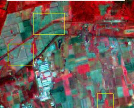
(f). Predicted LISS III for 17-Nov-2012 using proposed method

Table 2. Quantitative Comparison of the Proposed Method against SH Method for the Dataset: 2

Method	SSIM				RMSE				SAM
	B2	B3	B4	B5	B2	B3	B4	B5
Proposed method	0.9251	0.9034	0.8844	0.8735	0.0076	0.0111	0.0153	0.0131	2.2450
Song and Huang (2013)	0.9082	0.8736	0.8504	0.8350	0.0080	0.0124	0.0170	0.0147	2.5099

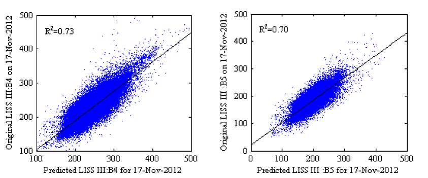
Fig.8. Scatter Plots of the Predicted Against the Actual Surface Reflectance of the Experimental Dataset: 2 for the Song and Huang (2013) Method

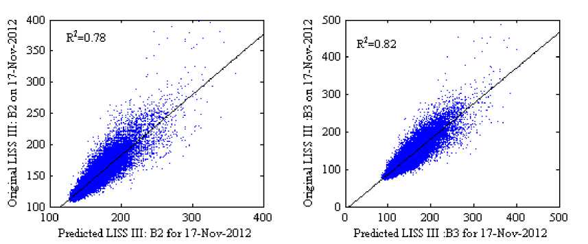
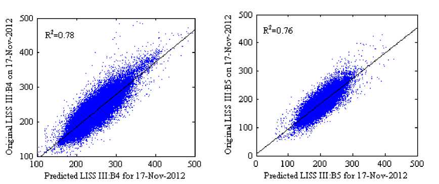
Fig.9. Scatter Plots of the Predicted Against the Actual Surface Reflectance of the Experimental Dataset: 2 for the Proposed Method

Although we have obtained a goodness of fit R2 between predicted and the actual surface reflectance values better than the Song and Huang (2013) method [21], still there is a need to improve the prediction accuracy. In prediction of land-cover-type changes, both Song and Huang (2013) [21] method and the proposed method were suffered to retrieve the actual surface reflectance. The prediction accuracy R2 for crop phenology changes is around 88% but for the land-cover-type changes is around 78%. By observing these quantitative and visual results, it is considerable evidence that as mentioned by Huang and Song (2012) [12] the accurate prediction of the land-cover-type changes is more difficult than the prediction of crop phenology changes.

• V.    C onclusion

We have proposed and demonstrated the spatiotemporal data fusion to create a synthetic LISS III image at time t^ with an AWiFS image at time t^ and a single AWiFS–LISS III image pair at time t0 , where t0 ≠ tk . The proposed method involves three phases, the first is super resolution phase, the second is high pass modulation phase, and the third is smoothing the spurious spatial discontinuities. In the first phase, two transition images are obtained by enhancing the spatial resolution of AWiFS image at time t0 and tk through single-image-super resolution technique. It requires a prior knowledge about the desired high resolution image. This prior knowledge is obtained through a single AWiFS–LISS III image pair at time t0 . The image patches of AWiFS–LISS III image pair are used to train the low and high resolution dictionaries with K-SVD algorithm, and the corresponding sparse coefficients are approximated with OMP. For a given low resolution AWiFS image patch of time tk , the sparse coefficients are obtained through the sparse coding technique OMP. The same sparse coefficients are used to derive the corresponding high resolution image patch for the time tk by using the high resolution dictionary. The derived high resolution images in the super resolution phase are called as transition images for the time t0 and tk .

In high-pass-modulation phase, the high frequency details which are obtained in the difference of LISS III image and the transition image of time t₀ , are proportionally injected into the transition image at time tk . In synthesis of multi-sensor and multi-temporal images, spurious spatial discontinuities are inevitable. Until now, no method has dealt with these spurious spatial discontinuities in spatiotemporal data fusion. In third phase of our method, we identified these spurious discontinuities and smoothed with the spatial-profileaveraging method.

Space borne global sensors have a trade-off between high spatial and high temporal resolutions. The proposed method can be used as an alternative to generate high spatial and high temporal images. With this approach, we can create a synthetic LISS III image at 23.5 m spatial and 5-day temporal resolutions. Although the proposed method captures crop phenology changes more similar to the original, still further improvement is required to predict the land-cover-type changes. Future work of this paper is to improve the prediction accuracy of the both crop phenology and land-cover-type changes.

A cknowledgement

This research was supported under technology development project (TDP) at National Remote Sensing Centre, ISRO, Department of Space, Government of India, through the project [0606313AE901].