Speaker Identification using SVM during Oriya Speech Recognition

Published Online September 2015 in MECS

In the last two decades, few Indian researchers have worked for the development of automatic speech recognition systems for Indian languages in such a way that development of this technology can reach at par with the research work which has been done for the different languages in the rest of the world.

The work in this paper is focused on establishing the duo tasks in the field of spoken engineering: speaker identification and speech recognition. Speaker identification task gives the information about the speaker i.e. “who has said it” and speech recognition task predicts “what has been said” by the speaker [2,4]. The conglomeration of duo techniques can be used for development of voice biometric-based speech recognizer. The traditional speech recognizer system only converts the input speech to text. But a voice biometric speech recognizer not only translates speech to text but also verifies the identity of the speaker.

The voice biometric-based speech recognizer in Oriya language consists of two key components i.e. speaker identification module and speech recognizer module. Both the modules are related to pattern recognition problems. Speaker identification module as well as speech recognizer module are developed by adopting stages like feature extraction, training for model generation and testing to use the generated model of training stage for requisite action as the end result. Multitudes of challenges are interfered during the system developments which are handled in different prospective ways. It is necessary to develop speech corpora in Oriya language for speech recognition and speaker identification as well. Feature selections are required for improving the accuracy rate of the system. In this work, gammatone frequency cepstral coefficients (GFCCs) are used in speaker identification module and mel-frequency cepstral coefficients (MFCCs) along with its first as well as second derivatives are used in Oriya speech recognizer module.

Multiple aspects are taken into account in this paper. Statistical pattern recognition algorithms are utilized in the development of speaker identification and Oriya speech recognition. Speaker identification task is based on the Support Vector Machine (SVM) algorithm whereas Hidden Markov Model (HMM) algorithm is used in Oriya speech recognition engine development.

Voice biometric-based speech recognizer has application in human computer interaction (HCI) system that assesses the user’s identity to perform any kind of transactions in Oriya language. The transaction is granted only if speaker's identity is found as valid one. This paper is organized as follows sec. 2 floats the background of voice recognition system, sec. 3 describes the speech database for speaker identification as well as Oriya speech recognition, sec.4 depicts the feature vectors generation, sec. 5 illustrates the pattern recognition algorithms for system development, sec. 6 emphasize on practical experimental results and sec. 7 conclusion and future work.

• II.    Background

The speech recognizer can be classified into different types namely, isolated speech recognizer, continuous speech recognizer, connected recognizer and spontaneous speech recognizer. The classification is based on the nature of audio files that can be handled by recognizer.

The development of speech recognition system is classified into five generations. Generation1 (1930 to 1950) speech recognizer was based on adhoc method to recognize sound or small vocabularies of isolated words. Generation2 (1950 to 1960) speech recognizer used acoustic phonetic approaches to recognize phonemes, phone or digit vocabularies. Generation3 (1960 to 1980) speech recognizer utilized pattern recognition techniques like linear predictive coding (LPC), vector quantization code book methods and dynamic programming methods with small to medium-sized vocabularies of isolated and connected sequences. Generation4 (1980 to 2000) speech recognizer was based on hidden Makov model that could handle continuous speech. Generation5(2000 to 2020) zeroed on parallel processing methods to increase recognition decision reliability, combination of HMMs and acoustic phonetic approaches to detect and correct linguistic irregularities and that will also increase robustness for recognition of speech in noise.

The early attempt research in speech recognition was to develop isolated word recognizer and connected word recognizer. After getting a success milestone in isolated and connected speech recognizer developments, the next attempt was to develop continuous and spontaneous speech recognizers that provoked the researchers to shift in technology from template-based approaches to statistical modelling methods, especially the hidden Markov model approach. Since then, hidden Markov model techniques have become widely applied in every spheres of voice recognition system.

Projects and the INRS 86,000-word isolated word recognition system in Canada as well as the Philips rail information system, the CSELT system for Eurorail information ser-vices, the University of Duisburg, the Cambridge University systems, and the LIMSI voice recognition in Europe, are examples of the current activity in speech recognition research. Large vocabulary recognition systems are being developed based on the concept of interpreting telephony and telephone directory assistance in Japan. Syllable-recognisers have been designed to handle large vocabulary Mandarin dictation in China and Taiwan [3].

Speech recognition systems have been developed for array of applications such as telecommunications where a speech recognition system can provide information or access to data or services over the telephone line, in manufacturing, a recognition capability is provided to aid in the manufacturing processes. Other applications include the use of speech recognition in toys and games.

A lot of contributions were dedicated by speech processing scientists and researchers throughout the globe for English and non-English spoken languages. But very scanty research in Oriya spoken language is done so far. This research work is completely a novel contribution towards the Oriya language which is one of the recognized Indian official languages.

The impact of voice based biometric system is magnified at the time it is being merged with speech recognition system. The hybridization of speech recognition and speaker identification will be useful to extract private and vital information in proper authorized approach.

This system is very helpful in applications that validate the users from uttered speech at the beginning and then accept the speech input in Oriya language for manmachine communication. So, the entitled research work will hybridize the two distinct speech processing phenomena for providing multitudes of benefits to the end users.

• III.    Database establishment for speaker identification and speech Recognition

Speech database used in speaker identification consists of Oriya spoken phrases uttered by 50 speakers of both the genders. This database was recorded by taking Oriya speakers aged between 18 and 50 years old. Userdependent pass-phrase, prompted phrase and unique passphrase were used to record voice from the speakers in Oriya language. Three-fourth of speaker identification database was used for training and remaining one-fourth of speech files were used for testing purpose for identifying the speakers.

Oriya speech recognition corpus was collected from Oriya speaking persons of both genders. Most of the speakers were having Mogalbandi accent and few speakers were having Sambalpuri accent. These two variants of accents were used to handle the speech variability of spoken Oriya language. All the speakers were native Oriya speakers with no speech impediments and were comfortable with the idea of having their speech recorded. The content of Oriya speech corpus is related to the college library. College library domain is taken into account because our motive is to use the research end product for academic purpose where students are going to access college library books through voice input after getting authorization from speaker identification mechanism.

Speech database meant for Oriya speech recognition and speaker identification were recorded in sampling rate of 16000Hz with quantization rate 16bit and mono channel. All the speech files were saved in wav formats.

• IV.    Feature vectors generation

CASA system incorporates a series of gammatone filters of T-F analysis. The gammatone filters are standard model of cochlear filtering and generated from psychophysical observations [5].

ℎ( t )= t^{a 1} ехр(-2πbt) cos(2πf_ct + φ). (1)

In the above Equation 1, a, b indicate the filter, t is time, fc is the filter’s center frequency, and φ is the phase, and a=4 is the order of the filter, b is the rectangular bandwidth ERB ( fs ) which increases with the center frequency fc . Glasberg and Moore have summarized human data on the equivalent rectangular bandwidth (ERB) of the auditory filter with the function:

ERB( fc ) = fc / Q + b₀ , (2) Bo = 24 .7

Q=9 .64498

where Bq is minimum bandwidth; Q is the asymptotic filter quality at large frequencies.

The filter output retains original sampling frequency. The 128 channel responses are down sampled to 100 Hz along the time dimension. The magnitudes of the downsampled outputs are then loudness-compressed by a cubic root operation. The resulting responses Gc [ m ] form a matrix, representing a T-F decomposition of the input, m is the frame index and c is the channel index. This T-F represents cochleagram, analogous to the widely used spectrogram. A cochleagram provides a much higher frequency resolution at low frequencies than at high frequencies. The T-F of cochleargram is a GF feature. Discrete cosine transform (DCT) is applied over GF feature that reduces the dimensionality and de-correlate its components. The resulting coefficients are called gammatone frequency cepstral coefficients GFCCs [6, 7, 8].

• V.    voice biometric-based speech recognizer

ARCHITECTURE

In this research article, we have conglomerated the speaker identification module with Oriya speech recognizer. So, the hybridized system will be helpful in man-machine communication in Oriya language with proper authentication at the beginning of communication. The communication in this research work is between students and machine. Students validate themselves through their voices using speaker identification technique and identified students are later allowed to get the information regarding the availability of books in the college library through speech recognition technique. Speaker identification module is developed using Support Vector Machine (SVM) and Oriya speech recognition is developed using Hidden Markov Model (HMM).

• A.    Support Vector Machine as Classifier for Speaker Identification

SVM classifier is superior in comparison to most of other classifiers because it proposes the solution with maximum margin that makes the classifier robust in comparison to others, SVM can handle input with very high dimensionality and it utilizes the optimization theory of duality to make estimation of model parameters in higher dimensional feature space computationally tractable. During the training procedure SVM creates model those are represented by samples placed in feature space where samples belonging to the same class are separated in feature space with a margin, which size is as much as possible. Unknown data are also mapped into this space and are classified based on the position in this feature space. Formally, we can say that SVM creates hyper plane or a collection of hyper planes in higherdimensional or infinite dimensional feature space. The best separation ability is achieved if hyper plane has the greatest distance from the nearest training samples of arbitrary class [9, 10].

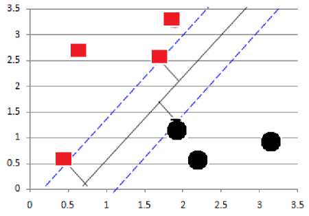
Fig.1. Two Classes of Observations with Maximal Marginal Hyperplane.

Fig. 1 is having two classes of observations, shown in circle and in square representation. The maximal margin hyperplane is shown as a solid line. The margin is the distance from the solid line to either of the dashed lines. It is also seen from Fig. 1 that, three training observations are equidistant from the maximal margin hyperplane and lie along the dashed lines indicating the width of the margin. These three observations are called as support vectors, because they “support” the maximal margin hyperplane that means if these points are moved slightly then the maximal margin hyperplane would move as well.

It is very peculiar and interesting phenomenon that, the maximal margin hyperplane depends directly on the support vectors, but not on the other observations.

The support vector classifier classifies a test observation depending on which side of a hyperplane it lies. The hyperplane is chosen to correctly separate most of the training observations into the two classes, but may misclassify a few observations [11, 12]. It is the solution to the optimization problem.

maximize M

Ро , Pl , Р2 ^,        Рр , , ^1 ^,        ^П ,

Subject to ∑ 7=1 Pj =1,

Vt ( Ро + Pl Xl + Рг ^2 +........+ Рр Хр ) ≥ м (1- ∈ I ),

∈ I ≥0,∑ "=1 ∈ I ≤ С              (3)

where C is a nonnegative tuning parameter. M is the width of the margin; we seek to make this quantity as large as possible. In Equation 3, ∈ Y , ∈ 2. . . , ∈ п are slack variables that allow individual observations to be on the wrong side of the margin or the hyperplane.

The fundamental approach of support vector classifier is for linear classification in the two-class setting but it can be extended to handle non-linear class boundaries. In that case, the support vector classifier addresses the problem of possibly non-linear boundaries between classes in a similar way, by enlarging the feature space using quadratic, cubic, and even higher-order polynomial functions of the predictors [13]. The Equation 3 would become maximize M

Ро , Р1 , Р2 , ……․ Рр , , ^1 , ……․ ^п , Subject to

• У1 ( Ро + ∑ j=lP]l^xij + ∑ ^=lPj2 4 ) ≥ М (1- ∈ I )

^∑ "=1 ∈ I ≤ С , ∈ I ≥0,∑7=1 ^∑ к=1 Р}к =1.    (4)

The kernel approach is an efficient computational approach to accommodate a non-linear boundary between the classes. Hence, the solution to the support vector classifier problem ( Equation 4) involves only the inner products of the observations. Thus the inner product of two observations ,   _, is given by

К ( х , x_t> , )= ∑ i=i ^хч , ^XU] ,            (5)

where K is kernel is a function that quantifies the similarity of two observations.

SVMs construct an optimal separation hyper plane in the higher dimensional space by choosing a nonlinear mapping. The mapping into higher dimensional space is performed by the kernel function К 〈 х , Х( _, 〉 . The kernel function allows us to map features from the original feature space into higher-dimensional feature space. The data can become linearly separable in feature space although original input is not linearly separable in the input space. In this research paper, we have used Radial Basis Function (RBF) as kernel function [14]

К ( х , x_t, _,)= ехр(-|| X - Xi )||²/ 2а² .     (6)

• B.    Bakis model of HMM as Oriya Speech Recognizer

HMM-based speech recognition acts as pattern recognition approach where a speech signal of spoken utterance is mapped to strings of meaningful words. Mapping a speech signal into meaningful words can be performed using multi-level pattern recognition, since the acoustic speech signals can be structured into a hierarchy of speech units such as sub-words (phonemes), words, and strings of words (sentences) [15].

The input speech signal collected through a microphone from user is converted into a sequence of fixed-size acoustic vectors Y = y 1 , · · ·, y T in a process called feature extraction. The decoder then attempts to find the sequence of words W = w 1 , · · ·, w K that is most likely to have generated Y, i. e., the decoder tries to find

^̂ = argmax [ р ( W | У )].           (7)

w

As p(W|Y) is difficult to model directly, Bayes' rule is used to transform Equation into the equivalent problem of finding:

^̂ = агдтах [ р ( У | W ) р ( W )].       (8)

w

• C.    Feature Extraction for Oriya Speech Recognizer

Feature extraction is consisting of signal processing algorithms that are used to extract salient feature vectors, maintaining the information necessary for recognition of speech and discarding the remainder which are unnecessary for current usability. This work is based on Mel-Frequency Cepstral Coefficients and added with local temporal dynamics of the speech signal to the feature representation for further improvement of speech recognition accuracy.

Feature vectors are normally calculated in every 10 ms using an overlapping analysis window of size nearly 25 ms. MFCCs are generated by applying a truncated discrete cosine transformation (DCT) to a log spectral estimate computed by smoothing an FFT with around 20 frequency bins distributed non-linearly across the speech spectrum. The non-linear frequency scale used is called a mel scale and it approximates the response of the human ear. The DCT is applied in order to smooth the spectral estimate and approximately decorrelate the feature elements. After the cosine transform the first element represents the average of the log-energy of the frequency bins [18].

In addition to the spectral coefficients, first order (delta) and second-order (delta–delta) regression coefficients are appended. If the original (static) feature vector is y t , then the delta parameter, ∆ys, is given by

∑ =1 Wi ( У, +1 ^- У, - ) ^∆ ^ ₌   =1 _{2 ∑} =1 ^{2     ,}

where n is the window width and wi are the regression coefficients. The delta–delta parameters, ∆2yt, are derived in the same fashion, but using differences of the delta parameters [19]. When concatenated together these form the feature vector yt, yt =[ У/ T Wt т ^Уf T]T (10)

In this paper, mel frequency cepstral coefficients and its first as well second derivatives are used. The final result is a feature vector whose dimensionality is typically around 40.

The likelihood p(Y|W) is determined by an acoustic model and the prior p(W) is determined by a language model [16]. The acoustic model is not normalized and the language model is often scaled by an empirically determined constant and a word-insertion penalty is added i.e. in the log domain the total likelihood is calculated as log p(Y|W) + α p(W) + β|W| where α is typically in the range 8–20 and β is typically in the range 0 to -20. The basic unit of sound represented by the acoustic model is the phone [17].

• D.    Acoustic model

The spoken words in W are represented in a sequence of basic sounds called base phones [20]. Words in a language may be pronounced in multiple pronunciation variation, the likelihood p(Y|W) can be computed over multiple pronunciation as

р (ПЮ= SqpC^IOpCQIWZ), (11)

where the summation is over all valid pronunciation sequences for W, Q is a particular sequence of pronunciations,

Р «Ж) = Ш = рРГО, (12)

and where each q^Wt is a valid pronunciation for word w_;. The summation in the Equation 12 is tractable as there will be very small number of alternative pronunciation for each of any language [21,22].

The individual phone q is represented by a continuous density HMM of the form illustrated in Fig. 2 with transition probability parameters {a ij } for transition from state s_i to state s j and output observation distributions {b j ()}.The acoustic model parameters λ = [{a_i j }, {b j ()}] can be efficiently estimated from a corpus of training utterances using the forward–backward algorithm.

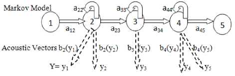
Fig.2. Phone Based HMM.

• E.    Trigram Language Model

Speech recognizer accuracy is greatly improved by taking the advantage of possible a priori information on the sequences to be recognized. The language model in speech recognizer takes the human centric approach as similar to a person recognizes the meaning of mispronounced word from the recognized words and of the meaning of the whole sentence. In this research paper, we have used stochastic models. The stochastic models are based on the joint probability of a word and its preceding words. The trigram probabilities are estimated by applying the maximum likelihood criterion, which corresponds to the frequency of occurrence of each 3-word sequence in the training speech transcriptions [21].

The trigram LM provides a probability of a complete word string W, given a two-word history:

(w) =

Р (w₁)P⁽W 2 ^|w₁⁾P⁽w₃^|W 2 W₁⁾......P(W n W _ м_ ₂) = П” = iPCw^Wi _ wi _ 2 ).            (13)

Probability is estimated using the relative frequency approach:

Р (w_i = w^m|w_i _ ! = w^m' , w ₂ _ ₂ = w^m' ' )

= ^(^5S;^^        (14)

• F.    Search method for Decoding

The search mechanism for statistical based speech recognition problems is to select the most probable string of words W among all possible word strings W for a given observation feature vector Xs. In this work, Sphinx4 decoder is used. It consists of three modules namely search manger, linguist and acoustic scorer. The fundamental motive of the search manger is to design and search a tree of possibilities for the best hypothesis generation. The design of the search tree is based on information obtained from the linguist. In the search process, each input feature frame is scored against the acoustic models. Depth-first search (DFS) or breadth-first search (BFS) is used to search the developed tree. Viterbi algorithm as well as Bush-derby algorithm is used in DFS or BFS data structure. During search process, phoneme or words (called competing units) are represented by directed graph. Each competing unit is assigned by the probability of best path and the unit that carries the maximum path score value will be selected by the search mechanism [23].

• VI. Practical Experimental Results

The experimental results in the current research work are carried out in three angles by looking at the fundamental units of developed system. First the system is exposed to measure the speaker identification accuracy using the GFCCs values from the speech signal by the pattern recognition technique called SVM and in second stage, the performance of Oriya speech recognition is measured using the HMM based on MFCC values from the speech signal. In the final stage, the speaker identification performance is evaluated by considering Oriya speech recognition service in speaker identification task.

• A. Evaluation of Speaker Identification using SVM

17.1982 16:-17.4899 17:-21.7531 18:-20.5923 19:3.8402 20:5.0810 21:3.4000 22:3.4126 23:4.4398 24:2.4048

Speech database for identification task described in section 2 is divided into two parts i.e. train and test database. The train database consists of 75% of speech utterance of individual speaker and remaining 25% was used as test database. Both databases were exposed to feature extraction process. In this research article, GFCCs are extracted from the speaker identification speech database meant for training as well as testing purposes. Fig. 3 shows the sample train data represented in GFCC.

1 1:15.1293 2:15.7980 3:17.9741 4:17.7398 5:22.6598

6:26.6554 7:27.2045 8:28.2281 9:30.1192 10:-9.5323

11:-11.2992 12:-10.1747 13:-11.3916 14:-16.9084 15:

25:-2.6766 26:-5.1613 27:-3.8503 28:-6.4786 29:-3.9945 30:-5.7855 31:-7.1301 32:-7.8418 33:-5.5834 34:-6.0906 35:-2.9635 36:-0.2366 37:-1.1812 38:4.7713 39:1.8064 40:6.0830 41:12.6563 42:10.1051 43:8.6079 44:9.4709 45:13.6614 46:-4.1768 47:-2.6238 48:-7.3882 49:-7.6976 50:-3.2320 51:-5.2043  52:-11.2827 53:-15.7638  54:7.1618  55:0.5755  56:1.1417  57:-1.5960  58:-2.7773

59:3.2133 60:-3.1038 61:-8.9570 62:-2.3924 63:1.7843 64:-0.8804 65:-1.7437 66:-3.4889 67:-2.2970 68:2.9593 69:10.3329 70:10.0460 71:4.8069 72:4.7267

2 1:22.7811 2:21.7612 3:50.8281 4:47.8177 5:20.0132 6:18.4138 7:6.8818 10:-4.0461 11:-2.6748 12:-4.3029 13:-4.3809    14:-8.8028    15:-11.9300   16:-11.4164

19:2.5083 20:4.6951 21:0.0136 22:-0.0656 23:-0.7138 24:-1.1745 25:2.3597 28:-0.6700 29:0.0053 30:-0.8789 31:-0.9494 32:-2.1105 33:-1.3494 34:1.7131 37:1.9603 38:0.6549 39:0.0108 40:-0.0525 41:3.0488 42:-0.7882 43:-4.6119 46:0.7041 47:1.0374 48:-0.3945 49:-0.4581 50:0.5270 51:2.2701 52:3.4990 55:-0.0408 56:0.3130 57:0.0989 58:0.0410 59:-2.5151 60:1.5504 61:4.0147 64:1.2033 65:1.5187 66:-0.2168 67:-0.2728 68:-0.6526 69:4.1969 70:4.8735 73:0.5928

• Fig.3.    Sample of GFCC Train Data

The values in the Fig. 3 indicate about the speaker identity and remaining describes about the GFCC values which are sequentially numbered. The speaker identity is assigned by numeral values starting from the integer 1 which is set for first speaker and integer value 2 is meant for second speaker in training stage. Fig. 3 illustrates about sample of two speakers where the voice data are represent as vector of real numbers. The transformation of voice data into real numbers is carried out using GFCC.

• 1)    Pre-processing data

Scaling operation is applied as pre-processing operation before applying SVM classifier. This is very crucial because it avoids attributes in greater numeric ranges dominating attributes of smaller ranges of numeric values. Scaling operation also transfers the data into such a representation that will be easier for processing by kernel functions. Each attribute of training and testing data is scaled to the range [-1, +1] for usability by SVM classifier. The optimization methods for training over preprocessing training data will take less time. Fig. 4 represents sample of pre-processed data i.e. scaled version of original train data.

1 1:0.0424363 2:-0.689974 3:-0.450074 4:-0.593571 5:0.70822 6:-0.166604 7:-0.13753 8:-0.0372342 9:0.0263057 10:-0.199589 11:0.415061 12:0.512529 13:0.282007 14:-0.26802 15:-0.305957 16:-0.363243 17:1 18:-1 19:0.201652 20:1 21:0.578562 22:0.200159 23:0.417272 24:0.18197 25:-0.0326957 26:-0.404849 27:-0.357618 28:-1 29:-0.689716 30:-0.736813 31:0.593151 32:-0.825968 33:-0.532495 34:-0.685003 35:0.376531 36:-0.15599 37:-1 38:1 39:0.972256 40:0.803922 41:1 42:0.759155 43:0.151618 44:0.385729 45:1 46:-0.763034 47:-0.434785 48:-1 49:-1 50:-1 51:-1 52:-1 53:-1 54:-1 55:0.364867 56:-0.136451 57:0.0902797 58:0.080932 59:0.431033 60:-0.0454501 61:0.804426 62:0.390176 63:0.816191 64:0.0778995 65:0.291972 66:-0.271359 67:-0.565371 68:-0.0249542 69:0.853722 70:0.886773 71:0.223247 72:0.201467

2 1:0.363712 2:-0.364897 3:0.787952 4:0.568701 5:0.8396 6:-0.467446 7:-0.883657 8:-1 9:-1 10:1 11:1 12:0.895598 13:1 14:0.67047 15:0.492933 16:0.561693 17:1 18:1 19:-0.0256502 20:0.950768 21:0.237569 22:0.132804 23:-0.0491429 24:-0.140253 25:0.557398 26:0.320185 27:0.118542 28:-0.494713 29:-0.385979 30:-0.364782 31:-0.140036 32:-0.386534 33:-0.219593 34:-0.167216 35:-0.149712 36:-0.136682 37:-0.618597 38:0.238317 39:0.541677 40:-0.191228 41:-0.0201427 42:-0.476235 43:-0.765793 44:-0.347183 45:-0.0756034 46:0.191264 47:0.454384 48:0.0905504 49:0.172151 50:0.121487 51:0.434227 52:0.725725 53:0.577271 54:0.547912 55:0.282425 56:-0.212156 57:0.134528 58:0.394308 59:-0.0877517 60:0.611487 61:0.996349 62:0.793388 63:0.575107 64:0.437251 65:0.782234 66:0.315459 67:-0.253781 68:-0.458803 69:0.0155853 70:0.160411 71:-0.351755 72:-0.346353

• Fig.4.    Sample of Scaled Train Data

• 2)    Train model using SVM

Radial basis function (RBF) is used as kernel function in this paper for transferring the training data into a higher dimensional space and also finds an optimal separation hyperplane in the higher dimensional space with a maximal margin. We have considered RBF kernel for model generation because this kernel function provides better flexibilities in the terms of less hyperparameters as well as less numerical difficulties in comparison to other kernel functions. Fig. 5 shows the sample train model generated by RBF kernel.

solver_type L2R_L2LOSS_SVC_DUAL nr_class 50

label 1 2 3....

nr_feature 117

bias -1

w

-0.02821990915031444

0.03108915575651317 0.01470233032503145 0.09022505984728009 0.006114697130436493 0.03040060825383623 0.01891424819599742 0.06962791001293467 0.02817967557251489 0.02723933650361284 0.05313289308612292 0.06117391797032717

0.0008231996514377281 0.04168810372621051

-0.01361236760688255

-0.05547561657468325-

0.0488195643953266-

0.03210152378387616

-0.07042669089854606

0.02048926370605698-

-0.02535058261379246

-0.03427790078985255-

0.04738940722675426-

-0.04205674818220831

-0.006820618584958762-

0.04765769571614877

-0.06473831246761264

Fig.5. Sample of SVM Based Train Model

• 3)    Test data

0.336798 42:-0.748256 43:-0.758617 44:-0.655394 45:0.638993 46:0.55647 47:2.17674 48:1.37351 49:0.725724 50:-1.83042 51:-0.614579 52:0.0302609 53:0.605437 54:1.09322 55:0.653633 56:-0.587236 57:0.687519 58:0.55337 59:0.497507 60:1.21507 61:1.57587 62:2.07634 63:1.44567 64:-1.58439 65:0.600881 66:-1.42586 67:-0.979742 68:-0.250317 69:1.19892 70:-1.2875 71:-0.734132 72:-0.105213

Testing of data is applied to identify the unknown speaker’s voice. First, the unknown voice is represented in GFCC and then it is scaled down into the same range of training data set. Finally the test utterance is identified using the SVM classifier. Fig. 6 represents the sample GFCC values of test voices. The first value in the Fig. 6 represents class label i.e. speaker identity and remaining values are represented in pair i.e. index: GFCC value.

1 1:0.778304 2:0.499563 3:0.409633 4:0.321566 5:0.274704 6:0.417682 7:0.440894 8:0.459887 9:0.452231 10:-0.421612 11:0.18364 12:0.228473 13:0.115984 14:-0.215929 15:-0.318952 16:-0.240436 17:0.623208 18:-0.675558 19:1.40795 20:2.5485 21:1.88121 22:1.47092 23:1.49485 24:1.52679 25:2.3415 26:2.73162 27:2.36247 28:0.285469 29:0.465046 30:0.308309 31:0.524195 32:0.145007 33:0.367789 34:-0.00130381 35:0.314505 36:0.324874 37:-0.919956 38:1.29545 39:1.09424 40:0.361745 41:-0.0169466 42:0.164896 43:0.0132964 44:0.109083 45:0.266877 46:1.01273 47:2.99301 48:1.61076 49:1.98874 50:3.63643 51:2.0063 52:1.19839 53:1.61041 54:2.91283 55:0.962505 56:0.147779 57:-0.00650587 58:-0.0251908 59:0.218136 60:-0.25812 61:-0.378183 62:-0.0551206 63:-0.0586328 64:1.01049 65:2.07167 66:1.32041 67:0.894125 68:0.769665 69:0.383459 70:1.0389 71:0.656296

2 1:1.08478 2:0.847427 3:0.688813 4:0.631239 5:0.678301 6:0.723112 7:0.744063 8:0.659776 9:0.601969 10:0.839048 11:0.96914 12:0.914589 13:0.691929 14:0.578353 15:0.593215 16:0.292078 17:0.133466 18:-0.0895529 19:0.298928 20:0.838423 21:0.288702 22:0.162327 23:0.676806 24:0.928323 25:1.83838 26:2.17915 27:1.82086 28:-0.335583 29:0.612624 30:-0.0319668 31:0.51841 32:0.626274 33:0.73087 34:0.523676 35:0.696382 36:0.93128 37:0.520985 38:1.24732 39:2.28119 40:0.994274 41:-

• Fig.6.    Sample of GFCC Test Data

• 4)    Scaled test data

After the extraction of GFCCs values from unknown speaker’s speech utterance, it is scaled to the same range as that of scaled version of training data. We have used same scaling factors for training and testing sets to obtain much accuracy in speaker identification task. Fig. 7 represents the sample of scaled version feature vectors of test speaker sets.

1 1:-1 2:-0.629582 3:-0.483223 4:-0.797322 5:-0.853842 6:-1 7:-1 8:-1 9:-1 10:-1 11:-1 12:-1 13:-1 14:-1 15:-1 16:1 17:-1 18:-1 19:1 20:1 21:1 22:1 23:1 24:1 25:1 26:1 27:1 28:1 29:1 30:1 31:1 32:0.126479 33:0.419301 34:0.256245 35:0.52242 36:0.293022 37:0.428069 38:1 39:0.473602 40:0.653339 41:1 42:1 43:1 44:1 45:1 46:0.945153 47:1 48:1 49:1 50:1 51:1 52:1 53:1 54:1 55:1 56:1 57:1 58:-1 59:-0.526486 60:-1 61:-1 62:-1 63:1 64:1 65:1 66:1 67:1 68:1 69:0.582985 70:1 71:1

2 1:1 2:1 3:1 4:1 5:1 6:1 7:1 8:1 9:1 10:0.568374 11:0.365035 12:0.173622 13:-0.166157 14:-0.284135 15:-0.39854 16:-0.629667 17:-0.373915 18:-0.329697 19:-1 20:-1 21:-1 22:-1 23:-0.672987 24:0.0435571 25:0.32243 26:0.400354 27:0.541996 28:-1 29:-1 30:0.246507 31:0.980312 32:1 33:1 34:1 35:1 36:1 37:1 38:0.972304 39:1 40:1 41:0.706645 42:0.315253 43:0.0932539 44:0.186297 45:-0.136754 46:-1 47:0.119858 48:0.650182 49:-1 50:-1 51:-0.965393 52:0.759041 53:-0.396663 54:0.112768 55:-1 56:-1 57:0.760708 58:1 59:1 60:1 61:1 62:1 63:1 64:-1 65:-1 66:-1 67:-1 68:-1 69:-1 70:-1 71:-1 72:-1 73:1

• Fig.7.    Sample of Scaled Test Data

Table 1. Result of Speaker Identification task using SVM

Speaker Id	Total Sample	No. Of Correct Acceptance	No. of False Acceptance	Accuracy Rate
1	10	7	3	70
2	10	8	2	80
3	10	7	3	70
4	10	6	4	60
5	10	9	1	90
6	10	7	3	70
7	10	5	5	50
8	10	8	2	80
9	10	7	3	70
10	10	6	4	60

Table1 shows the speaker identification result of SVM classifier using RBF kernel function based on GFCCs values. The result is calculated by considering ten speaker randomly from the test speech database and we have also considered ten utterance related to voice password for each speaker.

The average performance evaluation of Speaker Identification of SVM is found as 70%. The correct acceptance and false acceptance are measured by comparing the class label values of test data set and SVM classifiers predicted values.

• B.    Performance of Oriya Speech Recognizer

In this research we evaluated Oriya speech recognizer using left -to- right model of HMM which allows the states to move to themselves or to successive states but prevents to transit previous states. HMM transcribes the Oriya spoken utterances as the output of finite state machines. We have used phoneme based Oriya word and sentence recognition. In this current work, three emitting states of HMM with seven Gaussian mixtures are utilized. HMM based speech recognizer was trained using speech database that contained the Oriya isolated words as well as sentences related to college library system. The HMM based Oriya speech recognizer tool was evaluated using ten seen users and ten unseen users. The decoder used in Oriya speech recognition system is based on Sphinx4. Word and sentence accuracy are shown in Table 2 by considering ten seen users and unseen users. The word accuracy and sentence accuracy rate are calculated as Equation 15 and Equation 16.

word. Accuracy =         ∗ 100,      (15)

where N, D, S and I represent total number of words in test data, number of substitution errors and deletion errors and insertion errors respectively.

Number of sentence recognized correctly Sentence Accuracy =                                      *100

Number of sentence in test suit

Table 2. Accuracy Rate of Oriya Speech Recognizer.

Category of User	Word Accuracy (%)	Sentence Accuracy (%)
Seen Users	94.72	73. 54
Unseen Users	78.23	57.83

• C.    Oriya Speech Recognition Followed by Identification

The speaker identification accuracy rate is enhanced by using the speech recognition methodology in identification task. The spoken audio file of the user is first transcribed by the ASR which converts the spoken input into word. The transcribed text is then used to find the closest matches from the database which contained the textual data of audio files used during speaker identification training phase. Finally, the reference models corresponding to the closest matches are used by SVM classifier to find the identity of the speaker. The speaker identification performance is measured by incorporating speech recognition technique and without speech recognition technique. The result is shown in the Table 3.

Table 3. Performance of Speaker Identification with/without Speech Recognizer

category	True Acceptance (%)	False Acceptance (%)
SID using only SVM	70	30
speech recognition + identification (SVM)	75	25

• VII. Conclusion And Future Work

This research paper is based on spoken language engineering methodology to develop an efficient speech recognizer in Oriya language as well as identify the speakers more accurately. Humans are very intelligent in understanding the spoken language and identifying the voice of speakers. So, we have incorporated natural abilities of human beings in Oriya spoken language research that achieved mindboggling successful result. GFCCs were chosen as feature vectors for speaker identification task as it was found that GFCC performs comparatively better than other features in noisy condition. But mel-frequency cepstral coefficients and its variants namely delta as well as delta-delta accelerations were used during Oriya speech recognition which accorded with the suggested and commonly used features in speech recognition. SVM with RBF kernel was used for speaker identification algorithm but Bakis model of HMM with three transitional states was used for Oriya speech recognition. The accuracy of the speaker identification result was found as 70% using SVM. The accuracy rate of Oriya speech recognizer was represented in word accuracy and sentence accuracy rate for seen and unseen users. The word accuracy for seen and unseen users was found as 94.72% and 78.23% respectively where as the sentence accuracy was found as 73. 54% for seen users and 57.83% for unseen users. The performance of speaker identification was improved by adopting Oriya speech recognizer that acted as speaker pruning which ultimately increased the accuracy rate from 70% to 75%. Linguistic information and lexical characteristics of speakers will be included in future work for enhancement of accuracy rate of speaker identification task. Due to the lack of mimicry voice availability, the current research work does not focus its performance against the disguise voices. So, the work will be extended in future to handle the mimicry problem during speaker identification. Prosody is not used in development process of current Oriya ASR. The use of prosody will improve the performance of automatic speech recognizer because prosody is related to syntax, semantics, discourse and pragmatics. So, it will be included in near future. Moreover, in future, dynamically varying pronunciation models will be used in the architecture of Oriya ASR in order to deal with non-native speakers of Oriya language.