Spectral and Time Based Assessment of Meditative Heart Rate Signals

Published Online April 2013 in MECS DOI: 10.5815/ijigsp.2013.04.01

Meditation refers to a family of mental training practices that is designed to familiarize the practitioner with specific types of mental processes [1]. Meditation is a physiological state of demonstrated reduced metabolic activity – different from sleep – that elicits physical and mental relaxation and it is reported to enhance psychological balance and emotional stability [2]. In addition, meditation is recommended as nonmedicated treatment for some psychological disorders because, unlike medication, meditation has no side effects.

A large number of studies aimed at studying observed effects of meditation on heart rate signals [3-7]. Heart rate variability (HRV) can be described as variation of R-R intervals with respect to the time or beat number. HRV that is a nonstationary signal gives information about parasympathetic and sympathetic activity of autonomic nervous system (ANS) [8-9].

Previously [10-11], power spectral density (PSD) distribution of HRV signals was integrated in the very low-frequency band (VLF), (0-0.03 Hz), the low-frequency band (LF) (0.04–0.15 Hz) and the high-frequency band (HF) (0.15–0.4 Hz). It has shown that

VLF caused by thermoregulation and humoral factors; LF comes from baroreflex-related heart rate variability; and the HF arises from the respiratory sinus arrhythmia (RSA).

Eigenvector methods are used for estimating frequencies and powers of signals from noisecorrupted measurements. These methods are based on an eigen-decomposition of the correlation matrix of the noisecorrupted signal. Even when the signal-to-noise ratio (SNR) is low, the eigenvector methods produce frequency spectra of high resolution. These methods are best suited to signals that can be assumed to be composed of several specific sinusoids buried in noise [12-13]. In this study, some eigenvector methods (e.g. pisarenko, multiple signal classification (MUSIC), and minimum-norm) were selected to generate the PSD estimates. In addition, the Autoregressive (AR), ML-Capon, Periodogram, methods are employed to determine PSDs of heart rate signals during two states: before meditation and during meditation.

A number of spectral estimation techniques have recently been developed and have been compared to the more standard fast fourier transform (FFT) method, for biomedical signal processing [13-16]. FFT-based power spectrum estimation methods are known as classical methods and have been widely studied in the literature [17]. Autoregressive moving average (ARMA) and AR methods are model-based (parametric) methods.

ARMA model is the most general and important tool of modeling system. However, the main difficulty to use this method is the estimation of the optimum model order [18–20]. Accordingly, some algorithms were proposed to solve this problem, such as the final prediction error (FPE) and the Akaike’s information criterion [21,22], the Parzen’s criterion of autoregressive transfer function [23], and the Rissanen’s minimum description length method (MDL) [24].

In this study, The RR interval data were analyzed in terms of HRV parameters both in time domain and frequency domain. In addition, it is concerned with finding adequate ARMA model orders for spectral analysis of short segments of the time series formed from RR intervals. Jones [25] noted that Akaike’s final prediction error (FPE) and Akaike’s information criterion (AIC) tend to predict identical model orders for the same frames of measured data. Therefore, in this article FPE is applied to estimate the identical model order.

The outline of current study is as follows. In the next section, the set of HRV signals used in this study is briefly described. Then, the computation of the ARMA model and the FPE is explained. Finally, the results of present study are shown and the study is concluded.

• B.    Time Domain Analysis

Consider two random variables, x and y that the joint probability function of which is given. Let a new random variable, z=f(x, y) , be a single valued function of these two variables. The expectation, E{z} , is defined [27] by:

E { z } = E { f ( x , У )} =         f ( x , У ) P ( x , У ) dxdy      ⁽¹⁾

-^ -Ю

• II.    BACKGROUND

• A. Data selection

In this study, we used heart rate signals from Physionet [26], of subjects prior and during meditation. These two types of signals are shown in Fig. 1. Subjects were considered to be at an advanced level of meditation training. The Chi meditators [26] were all graduate and post-doctoral students. They were also relative novices in their practice of Chi meditation, most of them having begun their meditation practice about 1 –3 months before this study. The subjects were in good general health and did not follow any specific exercise routines.

The eight Chi meditators, 5 women and 3 men (age range 26–35, mean 29 years), wore a Holter recorder for about 10 hours during which time they went about their ordinary daily activities. At approximately 5 hours into the recording each of them practiced one hour of meditation. Meditation beginning and ending times were delineated with event marks.

During these sessions, the Chi meditators sat quietly, listening to the taped guidance of the Master. The meditators were instructed to breathe spontaneously while visualizing the opening and closing of a perfect lotus in the stomach. The meditation session lasted about one hour. The sampling rate was 360 Hz. Analysis was performed offline and meditation beginning and ending times were delineated with event marks [26].

The expectation is also known as the statistical average or mean. If x and y are discrete such that x gets the values x_i, i=1, 2, …, I and y gets y j , j=1, 2, …, J, then the expectation is:

E { z } = E { f ( x , y )} = £ £ f ( X i , y j P ( x , y j )        (2)

i = 1 j = 1

It is easy to show that the expectation is a linear operator. For example, consider the function z=xⁿ . The expectation of xⁿ is known as the n^th moment of x :

+»

E { x ” } =     xⁿ p ( x ) dx

-»

The first moment of x , m=E{x} , is called the mean, which is similarly defined as (4):

Ц = E { x (t )}

The second central moment has a special importance; it is called the variance and is denoted by a .

a x = Ц 2 = E { ( x - m ) 2 } = f   ( x - m ) 2 P ( x ) dx        (5)

-»

The skewness and kurtosis are defined as (6) and (7), respectively:

E { ( x ( t ) - ц ) ³}/, E { ( x ( t ) - ц ) ⁴^

’ a3

’ a ⁴

Heart Rate Signals

Figure 1. Heart rate variability (record C1): (top) before meditation (bottom) during meditation.

P ( ® ) =

^л m

£ ^{w ( k} ) ^{e ,(} ® ) v k I²

( k = p + 1              )

where,

(1       MUSIC w (k) = 12( k)

( £ ( k - m )

Eigenvector Pisarenko

where 5 ( k ) is the Kronecker delta function.

The Pisarenko method proposed by Pisarenko [28] is particularly useful for estimating PSD which contains sharp peaks at the expected frequencies. The polynomial A(f) which contains zeros on the unit circle can then be used to estimate the PSD.

m

A ⁽ f ) = E ^ak ^exP^{( -} j^{2 n k} )                       (11)

k=o where A(f) represents the desired polynomial, ak represents coefficients of the desired polynomial, and m represents the order of the eigen filter, A(f).

The polynomial can also be expressed in terms of the autocorrelation matrix R of the input signal. Assuming that the noise is white:

R = E{ x ( n ) * . x ( n ) T } = SPS # + ov ² 1                (12)

where x(n) is observed signal, S represents the signal direction matrix of dimension (m+1) X L and L is the dimension of the signal subspace, R is the autocorrelation matrix of dimension (m+1) X (m+1) , P is the signal power matrix of dimension (L) X (L) , ov² represents the noise power, ∗ represents the complex conjugate, I is the identity matrix, # represents the complex conjugate transposed, T shows the matrix transposed. S , the signal direction matrix is expressed as

where w 1 , w 2 , … , w L represent the signal frequencies:

Sw i = [1 e jw X ^{2 wi} . e ^jmw ] T    i = 1,2, . , L      (14)

In practical applications, it is common to construct the estimated autocorrelation matrix Rˆ   from the autocorrelation lags:

, N - 1 - k

RR ( k ) = — У x ( n + k ) ■ x ( n ) k = 0,1, . , m         (15)

N n = 0

where k is the autocorrelation lag index and N is the number of the signal samples. Then, the estimated autocorrelation matrix becomes

T? ( k ) =	г ~ 1R (0) T R (1) :	R ˆ(1) R ˆ(0)	~      1 .   R ( m ) . R ( m - 1)	(16)
	[ R ( m )	R ( m - 1)  .	.     TR (0)   J

Multiplying by the eigenvector of the autocorrelation matrix a , (14) can be rewritten as

Ra = SPS # a + o v ² a                            (17)

where a represents the eigenvector of the estimated autocorrelation matrix Rˆ and a is expressed as a = [ a о a1 . am]T                                 (18)

The Pisarenko method uses only the eigenvector corresponding to the minimum eigenvalue to construct the desired polynomial (11) and to calculate the spectrum [28]. Thus, the Pisarenko method determines a such that S^#a=0 . The eigenvector a can then be considered to lie in the noise subspace, and (17) reduces to

7 R a = o v ² a                                          (19)

under the constraint a^#a =1 where σν² is the noise power which in the Pisarenko method is the same as the minimum eigenvalue corresponding to the eigenvector a .

In principle, under the assumption of white noise all noise subspace eigenvalues should be equal,

2 1 = ^ 2 = . = A K = ov ²                       (20)

where λ i represents the noise subspace eigenvalues, i = 1, 2, … , K and K represents the dimension of the noise subspace.

From the eigenvector corresponding to the minimum eigenvalue, the Pisarenko method determines the signal PSD from the desired polynomial:

^ppisarenkO. f ) =;----у                       ⁽²¹)

A ( f )²

The order m of the autocorrelation matrix R ^ˆ should be greater than, or equal to, the number of sinusoids L contained in the signal. However, this method, employing only the eigenvector corresponding to the minimum eigenvalue, may produce spurious zeros [12,28,29].

The multiple signal classification (MUSIC) method is also a noise subspace frequency estimator. The MUSIC method proposed by Schmidt [30] eliminates the effects of spurious zeros by using the averaged spectra of all of the eigenvectors corresponding to the noise subspace. The resultant PSD is determined from

P music ( f ) = -pK-v ------ (22)

• ¹    K El A i ( f )²

  /     i = 0

where K represents the dimension of noise subspace, A i (f) represents the desired polynomial that corresponds to all the eigenvectors of the noise subspace [12,28-30].

In addition to the Pisarenko and MUSIC methods, the Minimum-Norm method was investigated [12,23,29,31]. In order to differentiate spurious zeros from real zeros, the Minimum-Norm method forces spurious zeros inside the unit circle and calculates a desired noise subspace vector a from either the noise or signal subspace eigenvectors. Thus, while the Pisarenko method uses only the noise subspace eigenvector corresponding to the minimum eigenvalue, the Minimum-Norm method uses a linear combination of all noise subspace eigenvectors. Using the Minimum-Norm method, the polynomial A(f) is written as [31]

A (f) = Ai(f) A2( f)(23)

Where

L

A1( f) = 2 bke " j     b0 =1(24)

k = 0

m - L a2( f) = 2 CkZ"k  c 0 = 1(25)

k = 0

where b k and c k are the coefficients of the two polynomial components of A(f) . The polynomial A 1 (f) has L desired zeros on the unit circle while A 2 (f) has m -L spurious zeros. In order to force the zeros of A 2 (f) into the unit circle, A 2 (f) must be a minimum phase polynomial. The primary motivation behind the Minimum-Norm method is to construct A 2 (f) such that the value Q , defined below, will be minimum. This can be achieved by constructing A 2 (f) as a linear predictive filter [31]:

m

Q = £| ak\²  a 0 = 1                              (26)

k = 0

The polynomial A(f) can be estimated from either the signal subspace eigenvectors E s or from the noise subspace eigenvectors E n . These eigenvectors can be expressed as [32]

a = [

a ₀

E _n n  n n

]

a 0 = ¹

The resulting eigenvector a has the desired zeros on the unit circle and the spurious zeros inside the unit circle:

а = ^[ а 0 a a_m ^{f                              (31)}

The Minimum-Norm PSD can be estimated from a as follows [12,29,31]:

P min ( f ) =                                      (32)

A ( f ) ²

where K represents the dimension of the noise subspace.

The AR power spectrum is obtained as follows: First, a rank approximation of the matrix C is obtained, as C = VSV ' , where S is obtained from S by setting ^ (k) = 0, k = p + 1, . . ., M . The AR parameter vector is then obtained as the solution to (2a = 0 ; the method in [33] is used, and the solution is forced to have unity modulus.

The ML (Capon) solution is given by,

^PML ⁽ ® ) =

P

^ A ik) ।* '< “ ’ v‘\²

V k = 1

\-1

Let V denote the matrix of eigenvectors corresponding to the p largest eigenvalues of R . Partition matrix V as,

. V r

The AR parameter vector for the minimum-norm solution is given by (35).

E s

sT

E s ^'

E n

T n

E n ^'

- V r V 1 /(1 - V H V )

The power spectrum is given by (36).

S ( ® ) =

where s and n vectors consist of the first element of the signal and the noise subspace eigenvectors. E_s ^' and E_n ^' have the same elements of E_s and E_n , respectively, but with the first row deleted [32].

The desired eigenvector a can be constructed from either signal subspace eigenvectors or noise subspace eigenvectors:

p

1/ ^ a ( k )exp( - jk ® )

/  k = o

Periodogram can be defined as finding to discrete fourier transform (DFT) of datasets, taking the magnitude squared of the results and estimating the PSD [34]. This definition is presented mathematically as:

I" xx ( f ) =

X L ( f ) ^{2 f}s^L

a = ^[ /       , '0 ^]    a 0 = ¹

E s s /^{(1 -} s s )

where

L - 1

X L ( f ) = 2 X l [ n ] e ~^j2f / ^f s n = 0

where L is length of x L [n] signal and f s is sampling frequency. In practically, periodograms perform the N-point PSD estimate and is defined as:

Pxx (fk) = * XL (fkT ) , fk = f, k = 0,1,2,-, N -1 (39) fsL          N where

N - 1

X l ( f ) = Z ^Xl [ n ] e - j 2^ / N                  (40)

n = 0

• D.    Autoregressive moving Average (ARMA) Model

So far we have looked at nonparametric estimators. Parametric estimators are often useful, either because they lead to parsimonious estimates, or because the underlying physics of the problem suggest a parametric model.

The basic idea is that if x ( n ) depends upon a finite set of parameters, 9 , then all of its statistics can be expressed in terms of 9. For example, we obtain parametric estimates of the power spectrum by first estimating 9 , and then evaluating Pxxf 9 ).

The specific form we postulate for the relationship between 9 and the sequence x ( n ) constitutes a model. A popular model in time-series analysis is the AutoRegressive Moving-Average (ARMA) model,

Pq

x ( n ) = - ^ a ( k ) x ( n - k ) + ^ b ( k ) u ( n - k )           (41)

k = 1                 k = 0

where u ( n ) is assumed to be a sequence, with variance 2

a _u . The Auto-Regressive (AR) polynomial is defined by,

P

A ( z ) = £ a ( k ) z ^{- k}                              (42)

k = 0

where a(0) = 1 . A ( z ) is assumed to have all its roots inside the unit circle, that is, A(zo) = 0 ^ |zo| < 1 ; this condition is also referred to as the minimum-phase or causal and stable condition. In general, no restrictions need to be placed on the zeros of the Moving-Average (MA) polynomial,

q

B ( z ) = ^ a ( kb ) z ^{- k}                             (43)

k = 0

however, B ( z ) is usually assumed to be minimum-phase. The minimum-phase assumption is usually not true for discrete-time processes which are obtained by sampling a continuous-time process.

The power-spectrum of the ARMA process is given by (44),

_{P ( f} ) = _G 2 ^( z£

XX ^{( f} ) = ^UA ( z ) 2

_z = e 2 ^П

Note that the power spectrum does not retain any phase information about the transfer function H(z) = B(z)/A(z) . Since we do not have access to the sequence u(n) , one either assumes that u(n) has unit variance, or that b(0) = 1 . Instead of estimating Pxx( / ) V/e [-1/2,1/2] , as in the nonparametric approach, we have to estimate only (p + q + 1) parameters, namely, ^{ a ⁽ k ^)} kp = 1 , { b ⁽ k ^)} kp = 1 and u2 . .

Let h(n) denote the impulse response of the model in (41); hence, H(z) = B(z)/A(z) . The AR and MA parameters are related to the impulse response (IR) through,

n

^ a ( k ) h ( n - k ) = b ( n ) n e [ 0, q ]

k = 0

= 0, n ^ [ 0, q ]

In practice, the observed process is noisy, that is,

y (n )= x (n)+ w(n)

where process w(n) is additive colored Gaussian noise; the color of the noise is usually not known.

Given the noisy observed data, y(n) , we want to estimate the a(k) ’s and the b(k) ’s in (41). We assume that the model orders p and q are known. The determination of the model orders p and q is an important issue (routines AR order and MA order implement AR and MA model order determination techniques). In general, it is better to overestimate model orders rather than to underestimate them (however, specific implementations or algorithms may suffer from zero-divided-by-zero type problems).

• E)    FPE criterion

A different way of identifying ARMA models is by trial and error and use of a goodness-of-fit statistic. In this approach, a suite of candidate models are fit, and goodness-of-fit statistics are computed that penalize appropriately for excessive complexity. Final Prediction Error (FPE) and Akaike’s Information Theoretic Criterion (AIC) are two closely related alternative statistical measures of goodness-of-fit of an ARMA(p,q) model. Goodness of fit might be expected to be measured by some function of the variance of the model residuals: the fit improves as the residuals become smaller. Both the FPE and AIC are functions of the variance of residuals. Another factor that must be considered; however, is the number of estimated parameters. This is so because by including enough parameters we can force a model to perfectly fit any data set. Measures of goodness of fit must therefore compensate for the artificial improvement in fit that comes from increasing complexity of model structure.

Consider the sequence {S k } k=0, I, ,^,N-1 with its linear prediction of order ^~ p given by equation (47). Its prediction error is E p given by [27]

S k = - 1 м - 1 j = 1

1 N"Ч e ~ = N Is* +

k = 0

V

~ _p

I a j S k - 1 j = 1

It can be shown that the expectation of E ~ _p as N

approaches infinity is

~ i p+1

^{E { E} ~ ^} = 1 1 ^- "N " I ^G

Consider now another sequence {y k } infinitely long with the same statistical properties as {S(k)} . The predictor for this sequence will be

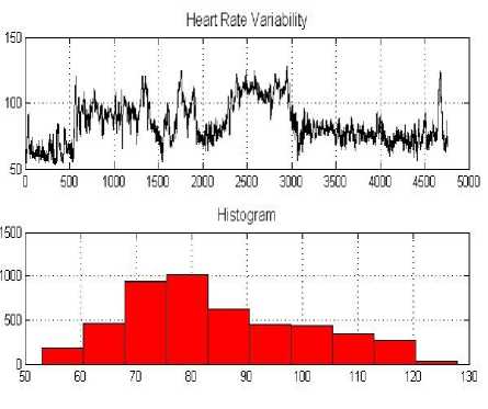
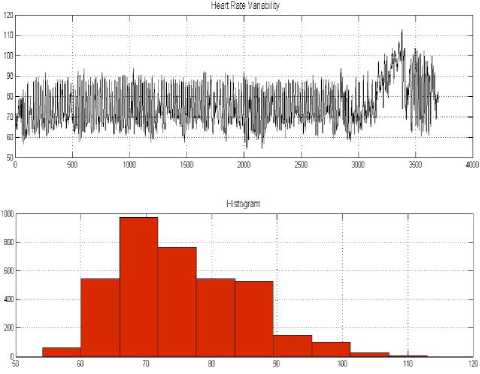
Fig. 2 (a) and Fig. 2 (b), show the data and the histogram before and during meditation, respectively. The mean, skewness, and kurtosis of signals in both conditions were estimated as shown in Figs. 3 to 5.

(a)

p

У k =^- I ^a j y * - 1 j = 1

where a j j = 1,2,..., p are functions of {S(k)} . The variance of the residuals tends asymptotically to ( 1 - ( ^p + 1 ) N ^{- 1} ) g ² as N approaches infinity. Hence, it is logical to estimate the FPE of the predictor (Equation (50)) by

~

FPE ( ~ ) =| 1 + p + 1 I G G"

V   n 7

Where G² is the variance of the input sequence {GU(k)} .

Since G² is not known, its estimate from equation (49) can be used such that

(b)

FPE (p ) =

1 + ^1

—-N r 1 - p + 1

V    N

E~

p

N + ~ + 1

N - p - 1 ^p

And the optimal model order  ~p is given by minimizing Equation (52).

FPE ( p ) = Min FPE ( p )                         (53)

~ _p

III. results

Heart rate signals - before and during meditation, are shown in Fig. 1. Obviously, the amplitude and frequency of heart rate signals are affected by meditation. According to Fig. 1, during meditation signals become more periodic and their chaotic behavior is decreased. The mean of heart rate signals also decreased during meditation.

Figure 2. Heart rate variability (record C4) and the histogram: (a) before meditation (b) during meditation.

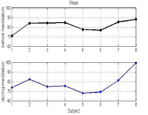
Figure 3. Mean of heart rate variability before and during meditation.

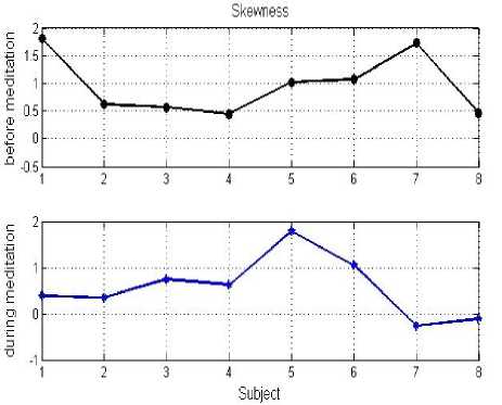
Figure 4. Skewness of heart rate variability before and during meditation.

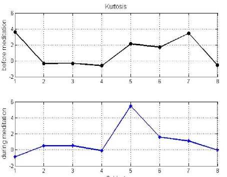
Figure 5. Kurtosis of heart rate variability before and during meditation.

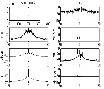
The (1,1) panel of Fig. 6 displays the singular values of the covariance matrix.

(b)

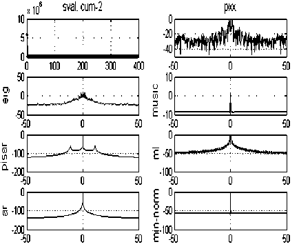
Figure 6. The singular values of the covariance matrix and the power spectrum estimations with different methods: (a) before meditation (b) during meditation

The number of harmonics can usually be determined by examining the singular value plot. The plot indicates that only one singular value is significant.

The number of dominant frequency components reflected by the peaks in the power spectrum.

According to Fig. 6, there is one peak in the power spectrum, corresponds to p=1. The corresponding power spectral estimates are shown in the remaining panels of Fig. 6: All of the estimates have a strong peak at about 0 Hz.

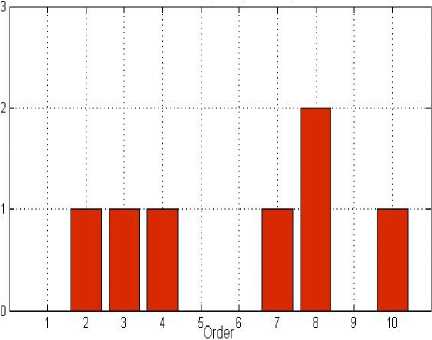
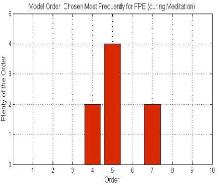
ARMA model of each signal with 10 different orders (1–10) were constructed and each data was tested using the criterion described above. In other words, the Akaike’s Final Prediction Error for each model was calculated. Then, the histogram of the optimum model order for the data was produced (Fig. 7).

(a)

Mod^ Oder Chosen Most Frequentlyfor FPE (6МадЙ№ЙЙ

(a)

(b)

Figure 7. The histogram of model order chosen most frequently for FPE (a) before meditation, (b) during meditation.

According to Fig. 7, it can be seen that overall the model order chosen most frequently for FPE was p = 8 for before meditation and p = 5 for during meditation.

• IV.    discussion

In this study, we investigate the heart rate variability during Chi meditation, in order to study the system behavior in different psychological states. The time domain and spectral measures of HRV from the R-R intervals were analyzed. Then, the HRV measures in meditation and rest were compared. Some measures in time domain including the mean heart rate and the second and third central moment of RR interval data were considered.

The AR, Eigenvector, ML-Capon, Periodogram, Pisarenko, MUSIC, and Minimum-Norm methods were employed to determine PSDs of heart rate signals during two states: before meditation and during meditation. The number of harmonics can usually be determined by examining the singular value plot (as shown in Fig. 6).

In all cases, the Pisarenko PSD showed extra peaks as compared to PSDs obtained from the other methods. Since the Pisarenko method showed tendency to generate spurious zeros, the Pisarenko was considered inappropriate for HRV signals. The MUSIC method eliminates these spurious zeros by averaging the spectra from all of the eigenvectors. The MUSIC method is the most widely applied in literatures as a result of simple computations and high-resolution [35-37]. The Minimum-Norm method treats the problem of spurious zeros by forcing them inside the unit circle. According to statistical analysis, the MUSIC method’s performance characteristics have been found to be superior to the Minimum-Norm method [38-41]. In PSD analysis, periodogram does not provide effective solution because of spectral leakage.

The selection of the model orders in the ARMA spectral estimator is a critical subject. Too low order results in a smoothed estimate, while too large order causes spurious peaks and general statistical instability. The ARMA spectral estimator offers the promise of higher resolution. When the dimension of the autocorrelation matrix is inappropriate and the model orders are chosen incorrect, poor spectral estimates are obtained by the ARMA model. Heavy biases and/or large variabilities may be exhibited. In this study, Akaike’s Final Prediction Error [27] was taken as the base for choosing the model order. According to the results, model order (p) was taken as 8 before meditation and 5 during meditation.

• V.    Conclusion

The results suggested that variety of orders in HRV models upon different psychological states could be due to some differences in intrinsic properties of the system. In other words, difference in ARMA model order was probably caused by individual differences in HRV.