Stability analysis of equilibrium points of newcastle disease model of village chicken in the presence of wild birds reservoir

Published Online April 2019 in MECS DOI: 10.5815/ijmsc.2019.02.01

(for n >  0) in a geometrical space [4, 11]. A steady state solution, X ( t ), is an equilibrium point of a dynamical system X' = M ( X , t ), X e K n if satisfies the condition M( X *,0) = 0, V t >  0 [11, 19, 21]. The solution X ( t ) of a dynamical system is stable if, for any arbitrarily small 8 >  0 , there exists 5 >  0 such that, for any trajectory X ( t ) for which || X (0) - X *(0)|| <  5 , then the inequality || X (0) - X *(0)|| <  8 is satisfied V t >  0 [19]. It is also stable iff all initial trajectories in an open set X e K ⁿ move towards X ( t ) and remain near it V t >  0 and is unstable if moves away from X ( t ) [21, 24, 25].

The steady state solution is referred as a disease free if the population is free from the disease whilst referred as the endemic if the disease persists in the population [16]. In this paper we study the existence and stability of both disease free equilibrium point (DFEP) and the endemic equilibrium point (EEP) of the Newcastle disease (ND) model developed by [6]. We apply a Hurwitz Matrix criterion to study the local stability of the disease free equilibrium point and the Castillo Chavez theorem [5] to study the global stability of the disease free equilibrium point. In addition, we apply the La Salle’s invariant principle and the Lyapunov method to study the stability of the endemic equilibrium point. Lastly, we use simulations to verify the analytical solutions of the ND model with environment and wild birds reservoirs. The motivation of this paper is to understand the existence and stability of the equilibrium points of the Newcastle disease model when wild birds are considered as the reservoir of the Newcastle disease virus. However, no study till yet in the field have considered the wild birds and environment as the secondary sources of ND.

• 2.    Related Works

Several stability analysis methods have been applied by different scholars when analyzing their epidemiological models [2, 16, 17, 18, 19, 21].

• [12]    used the trace and determinant method to study the local stability of the disease free equilibrium point of their models. In this method, the signs of trace and determinant of the variational Jacobian matrix decides the local stability of the disease free equilibrium point. [2] used the Lyapunov function to prove the global stability of the disease free equilibrium point of Dengue disease infection Model. [19] used a linearizion method to study the behavior of the disease free equilibrium point of a deterministic Epidemiological Model with Pseudorecovery. Additionally, [19] used a Lyapunov function method to study the stability of the endemic equilibrium point of his model. Moreover, [2, 17, 21] used Metzler matrix theorem to study local stability of the disease free equilibrium point of their models. Further, a Lyapunov method and the La Salle’s theorem are used by [21] to study the stability of the endemic equilibrium point of Malaria model. [16] used the Center Manifold theorem to study the global stability of the endemic equilibrium point of the Malaria model. In our model, the Hurwitz matrix criterion is applied to study the stability of the Newcastle disease free equilibrium point,

• 3.    Model Formulation

• 3.1.    Equations of the Model

In formulation of the model it is assumed that, the birth rate and death rate of the village chicken are the same. These populations are recruited at a constant birth дN (t) and д N^(t) with Nc (t) and Nw (t) as the total population of the village chicken and wild birds respectively. According to [6], the wild birds population N (t) is partitioned into susceptible S (t), exposed E (t) , the mildly infected wild birds I (t) and severely infected I (t) . The mild infected wild birds are not capable of transmitting the ND to other birds. The Village chicken population is partitioned into susceptible S (t) , exposed E (t) and the severely infected I (t) . The contaminated environment is denoted by H(t) The model assumed that the transmission of the NDV among the hosts is primarily through direct contact between the infected and susceptible chicken is the primary route for NDV while the contact of susceptible chicken with either contaminated environment or reservoir wild birds is the secondary route of the virus transmissions [7, 13]. Village chicken spread the ND virus after developing the clinical signs within the incubation period of two to fifteen days [1, 20, 23]. Furthermore, we assumed that the severely infected village chicken, severely infected wild birds, and the mildly infected wild birds all shed NDV into the environment at the rate α and α respectively. Other parameter of the model system

(1) Are described as in the table below;

Table 1. Parameters used for the ND Model System (1)

Parameter a b φ	Description Contact rate between the susceptible and mildly infected wild birds Contact rate between mildly infected wild birds and susceptible Chicken Contact rate between severely infected and susceptible wild birds Contact rate between severely infected and the susceptible chicken
ψ k d ρ	Contact rate between severely infected and susceptible chicken Half saturated constant of NDV in the environment Probability of chicken and wild birds to get infections from the environment Probability of the exposed wild bird to become severely infected
α c	Shading rate of NDV from severely infected village chicken to the environment
α w µ	Shading rate of NDV from mild and severe infected wild birds to the environment Recruitment rate and Natural mortality death rate of the hosts
µ v δ w	Clearance rate of the NDV from the environment Disease induced death rate in wild birds population
δ c γ	Disease induced death rate in the village chicken population Progression rate of ND for village chicken and wild birds

From the model flow descriptions found in [13], we have the following system of ODEs

^ = pN_c (i) - (ti-^ + b^ + ^7^ + m) SeW ^ = (^ + ⁶^ + S) ^S^ - ^ + ^(«) ^^ЕДО-^-ИШЦ

^ _{= pN}. (,) _ (№M0 ₊ ^ ₊ „) S₄t)

^ = (^t'^¹ + S) S„W " (7 + iWt)

^ = (l-phEw(t)-/1Jr(t)

^y = aJe^ + a. (/„(/) + Z_r(t)) - n.H(t')

with the initial conditions; S c (0) >  0, E_c (0) >  0, I c (0) >  0, S w (0) >  0 , E (0) >  0, I w (0) >  0, I r (0) >  0 ,

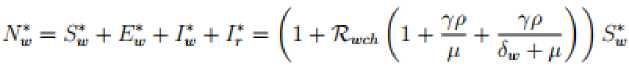
H(0) > 0, N(t) = Sc(t) + Ec(t) + Ic(t) and N*(t) = S(t) + E(t) + I*(t) + Ir (t)

• 4.    Analysis of the Model

  • 4.1.    t he b asic r eproduction n umber , R

As shown in [13], the Basic Reproduction Number of the model system (1) is;

• -          ,      ^f^       a(p-1)7 , ^„«„7(<$_w+^-/>($„)\

\   h+/i)(^w + M) (7 + Д)Д * (7 + w(^_W+^)M/*v /

/(у __££7__ д(р- 1)7 _ dN „n„7 (i.+li + p6.Y \² . *

'VX (7 + /C(^+/0 (7 + ^)m   Ц-f + MU^nJ

where

_Y _     *1 dN^ a_c

(7 + /j)(<$, + p) к (7+р)(<$с + д)/1„ д _      4 dN„у2 ac    / bNe (p - 1)   dNcOi», (6W + p + рб^

^K (7 + m) <& + p) Щ) \N_M (7 + P)P  ^K ("V + P) + p)Pp_v

• 4.2.    Equilibrium Points of the Model System

Proposition 4.1 The model system has two equilibrium points, disease free equilibrium point Q⁰ = { N c ,0,0, N_w ,0,0,0} and the endemic equilibrium point Q* = { S * , E * , I * , S ^ , E * ,I * ,I r , H } .

where

/• = _'^e;, e*_c = A5L, s: = ^L Oc-r P         p-r“f       Ре + P

Substituting S into E and E into I we get

• ⁶

r = 1 UPcN*

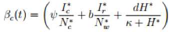
By considering the force of infections in chicken, I is obtained by solving the equation

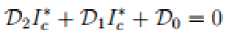
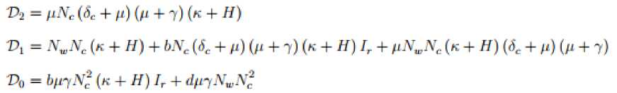
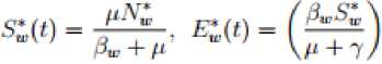
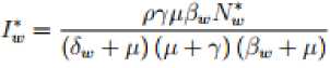
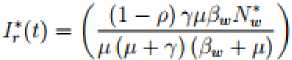
Where

Also in the wild birds population we have the following steady states;

Where 3W = (^WW + ^^y) and

7? _t = ^N-.h ^+149-+^

From equation (3) to (13) , the solution β = β = 0 gives the disease free equilibrium points while β ≠ 0and β ≠ 0 gives the endemic equilibrium point of the model in the system (1).

• 4.3.    Local stability of the Disease Free Equilibrium Point

The stability analysis of the disease free equilibrium point ( Q ⁰) of the model system (1) is examined by the Hurwitz Matrix criterion [22]. The Jacobian matrix J (q ⁰)is found by differentiating each equation of the model system w . r . t its state variables at Q ⁰ . Thus, the Jacobian matrix of the model system at Q ⁰ is then given by

	1-t*	0	-V	0	0	0	-b^	-d^
	0	-ji-7	*	0	0	0		d^
	0	7	— <$c — /4	0	0	0	0	0
w=	0	0	0	—[1	0	-p	—Й	-j^
	0	n	0	0	-ft - 7		ti	d!^
	0	0	0	0	P7	-&W — M	0	0
	0	0	0	0	(i - ph	0		0
	<0	0	de	0	0	№»	аш	-1^ ;

From matrix

(14) the

first

two

roots

of J ( Q ⁰ ) are

given by ( - д — 2 ) = 0 and ( - д - 2 ) = 0 . Then the

reduced (6 x 6) matrix become

with n = bN- , ₅ = dN c. and t = dNw

^Nw        ^{k         k}

Then characteristic polynomial for the matrix is defined as

G (A) = A⁶ + Bi A^s + B₂A⁴ + B₃A³ + B₄A² + B₅A + a₆

The corresponding Hurwitz matrix is then given by

'b_v B₃ B_s 0 0 0

1  B^ B3 Bs  о0

,      0  Bi  в3 в3  о0

Gif =

0   1  B4 Bl  Ba0

0   0  Bi  Bt Ba0

у 0   0    \  B₃  Bi  Ba j

where,

В_х = Pv + 3/1 + ф 4- 8_С 4- 7

• В,    = 7 р t + p_v 7 + 3 д» Р — Pv Ф + До 8_С + ар + и8_п, 4- 2 7 д — уф — уф — 7 / + 7 <5_С + 3 д² — Зфр + 2б_ср — ф6_с

Вл = Р»У pt + y²pt + 27 ppt 4- у pt8_c + p_vap 4- p«a8_w + 2p«y p — р„уф — реУФ — Ре 7 t + p„ 7 8_C 4- 3 p_e p² - 3 p_v p ф + 2 p„ p 8_C - р„ф8_с + у ap 4- ay 6_W 4- 3 ap² + 3ap 8_W 4- ap 8_C + a8_w 8_C — y²t 4- 7 p² — 2 7 рф—у рф — 27 pt + 7 p8_c + y фф — уф8_с — 7 sa_c — 7 t8_c 4- p³ — 3 р²ф 4- р²8_с — 2рф8_с

Вл = р»у²р1 4- 2р„у ppt 4- p_vypt6_c — 7³np — y²pnp 4- y²ppt — у²фpt — y²psa_w 4- y²p t8_c+y p²pt+y p pt8_c+Pt, 7 ap 4- pv ay 8_W 4-3 pe ap² 4-3 p„ap8_W 4-д_с ap 8_C 4- Pv a8_w 8_C — pey²t+pey p² —2p_vy рф—р_г,у рф—2 pt, у pt+p_ry p8_c+p_vy фф—fl,, у ф8_с — /^,7 td'_c4- pep³ — 3 fit,р²ф 4- р_г,p²8_c — 2p_vрф8_с + 2у ap² — ay рф +2ay p6_W 4- ay p8_C — ay ф6_W 4- ay 8_W 8_C 4- 3 up³ 4- 3 ap²8_W 4- 2 ap²8_c + 2ap 6_W 8_C 4- 7^Sr 4- y²p r — y²p t 4- у²ф t — y²t8_c — 7 р²ф — у p²t 4- 7 рфф — у рф8_с — у psa_c — ур t8_c 4- у фза_с — р³ф — р²ф8_с

Вц = 2 р„ ар 8_W 8_С 4- у²Ф р sa_w 4- у р Ф sa<, — p_v у²р пр 4- р_т у²р pt—p_e у² ф pt+p_v у²р t8_c 4- p_t, 7 р²рt — p-t, 7 ар ^4-2 р„ 7 ар8_W + р_гу ар8_С — р„у аф <$„ 4- p_v 7 ^и^«8_С + р_юу рФФ — р„ у рф8_с—реУ р t8_с—у²р stn_c—y up sa_c—y asa_c 8_W —2 y²p p sa_w—y p so#, 8_w—ay p ф d‘_w4- ay p 8e, 8_C-Vpt,ypp t8_c 4- 3 p„ up³ — p_x, р^лф 4- p_B y³n 4- 7³за_ш 4- ay p³ 4- ap³8_w 4- ap³8_c 4- ap⁴ — 7²sq_w 8ь — 7 p²sa_w + ay³np² — ay³np — ay р²ф 4- ay p²8_w 4- ay p²8_c 4- 3 /^ ap²8_w 42 pv ap²6_c — pv р²ф8_с — у^лр за_ш — p_v y³np 4- p_v y²p n — p_T y²p t 4- ре тФ I ~ До 7²^c + 2 p_e 7 ap² — pt, 7 р²ф — p_v у p²t 4- y²sta_c 4- ap²8_w 8_C

B₆ = pt, ap²8_w 8_C — y³p²8ta_w 4- y³p sta_w — 7 ap²sa_c 4- p_T y³arp² - p_v у^лагр — /a, 7 ар²ф 4- Pv 7 ap²8„ 4- p_u 7 ap²8_c — 7 ap sate 8_W — Pv У ap ф 8_W 4- p_T 7 ap 8_W 8_C 4- y²p ф p за_ш 4- p_T up¹ 4- Pt, ap³8_w-Vpeap³5_c+Pv 7 up³—a_w y²p²s—a_w 7 p³s—a_w y²p s8_w—a_m 7 р²н8_ш+у³ар²8а_п, — y³apsa_lw

The disease free equilibrium point is locally asymptotically stable iff the principal leading minors of G are all positive for n = 1, 2,..., 6.

Thus

	В,	B;t	S5	о
ag4 =	1	Вц	Вд	^
	о	Bi	Вд	Вд
	0	1	Ва	Вд

= B,B₂ (B₃B₄ — B₂B₄ + Вд^ + Вд (В₂ — Вд)

— Вд ^ВдВд — В2В5 + в^в^ + В;

	Bi Вд Вд
AG3 =	1 В2 Вд	= ВдВ^Вд — В^Вд — Вд + В1Вд.
	0 Bi Вд

	Bi	Вд	Вд	0	о	О
	1	в2	Вд	Ви	п	О
^Gfl =	О	Вт	Вд	Вд	О	о
	о	1	в.	Вд	в»	О
	О	0	Bl	Вд	Вт,	О
	О	О	1	В2	Вд	Bti

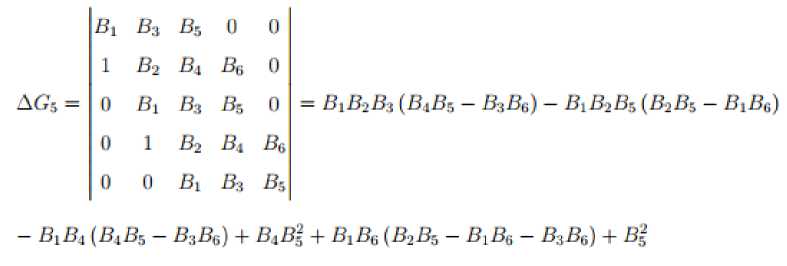
= ВхВ^ВдВдВ^Вб - В-’В* + В^ - В₆В» + 2В₆В,В₄В2 - В²₄В»В₆В_& - ЗВ^ВдВдВд + 2В²В²В_аВ₂ - ВдВ'^ВдВб + ВдВдВ^ + ВзВ₂В₆В? - ВбВхВ'^В! - BiBxB^B^.

t he disease free equilibrium point ( Q ⁰ ) of a model system (1) is LAS if

ДС_Ь ДСз, .... ДСб > 0. For ДС1 > 0 we have ц„ + 3 p 4- 6_C + 7 4- ф> 0, ДСз > 0 if В_|В.₂>В₃. AG₃>0if В₁В₂В_ЛА-В₁В₅> B²B₄A-B?_V Also ДС₄, ДС₅ and ДС₆ are grater than zero when B\B₂B₃B₄A- BxB₂B^ + В_лВ₂ + BiB₂B₄ + B^ > B₁B²B₄ + B² + B^B₄ + B_tB_лВ₄; В^В^ВдВ^В^ 4- В² B₂B₃B₆ + B₄B₃B₄B^ 4- B_tB^ + ВхВ₂В^В^ + В² > B₄B^B‘²B^ 4* В\В₂В² 4* В\В₄В₃ 4* В^В^ 4* В,В₃В^ ^ and В\В₂В_лВхВ₃Вц 4- В^В^ 4* 2B₆BiB₄B^ 4- 2В²В²В-₃В₂ 4- В₄В_ЛВ²В² 4- B_AB₂B_tiB3 4- В² В² > ЩВ'² 4- В^В^В₆В₅ 4- АВ^ВхВ₃В₃ 4~ В₄В₃В₃В^ — В^В\ В₂ В^ 4~ В₂В\В^В² respectively.

We therefore establish a theorem;

Theorem 4.1 G ( X ) is stable iff the leading principal minors of G_n (Forall n e ® ⁺ ) are all positive and thus the disease free equilibrium point is LAS .

• 4.4.    Global stability of the Disease Free Equilibrium Point

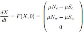
The global stability of the disease free equilibrium point of the ND model is done by the theorem as described by [5, 15, 16]. To apply the theorem, we write the model system (1) as;

d4-F^

^ = G(X,n,GW) = 0

Where X is the number of susceptible populations and I is the number of the infected populations whilst the disease free equilibrium point is given by Q⁰ = { X *, 0} . For the system (18) to be G . A.S , two conditions must be fulfilled;

• I.

• II.

d X            *

= F ( X 0) , X is globally asymptotically stable G . A . S , dt          ^,

G(X, I) = BI - (G(X, I), (G(X, I) > 0for(X, I) eQ where Q is the invariant region and B = DG (X;0) is an M -matrix with non-negative off diagonal elements. If the system (18) satisfies condition I and II below then the theorem below holds:

Theorem 4.2. A disease free equilibrium point ( Q ⁰) of a model described in system (1) is globally asymptotically stable G . A . S if R _o<  1 .

Proof;

We need to show that condition I and II holds when R_Q <  1. From the model system (1); the set of non-infectious classes is given by X = ( S_c , S ) e К 2 and for the infectious classes is given by I = ( E_c , I _c , E _w, I _w, I_r , H ) e К 6 . The model system (1) is then transferred into the form of the system (18) as follows

with Q⁰ = { N ,0,0, N_w ,0,0,0} . The system (19) is linear with the solutions S_c ( t ) = N_c + ( S_c (0) - N_c ) e ^ ‘ and Sw ( t ) = Nw + ( Sw (0) - Nw ) e-^ . It is obvious that

^Sc ⁽ t ) ^ ^Nc , S w ( t ) ^ N w as t ^ да depending on initial conditions. Thus, Q ⁰ is globally asymptotically stable and therefore condition I holds. Considering the condition number II we have;

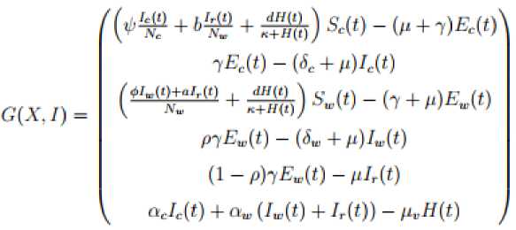
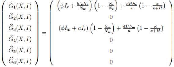
We need to show that, G (X, I) = BI - G (X, I), G (X, 0) > 0 for (X, I) e Q

The Jacobian matrix of equation (20) at Q ⁰ produces an M-matrix B as follows;

-p - 7 O 0 0 ^^ 7 —6C — // 0 0 0 0 0 0 -p - 7 0 fl ^^ B = 0 0 />7 — ^w  P 0 0 0 0 (i -ph 0 -p 0 0 ^w -Pv) and

f rom the matrix (21) , a matrix B comprises with all negative diagonal entries and all non-negative off-diagonal entries. Since N c ⁽ t ) = S c ⁽ t ) + E c ^(t ) + I c ⁽ t ) and N w ⁽ t ) = S w ⁽ t ) + E w ⁽ t ) + I w ⁽ t ) + I r ⁽ t ) , it is almost surely that S_c (0) <  N_c and S_w (0) <  N_w for { S_c ( t ), S_w ( t )} G Q and hence, in the matrix (22) we find that G, ( X , I ) >  0 and G ₃ ( X , I ) >  0.

Also G ₂ ( X , I ) = G 4 ( X , I ) = ( G 5 ( X , I ) = ( G ₆ ( X , I ) = 0. Hence, ( G , ( X ,0) >  0 for, where i = 1,2,...,6. Therefore condition II holds which shows that the disease free equilibrium point Q ⁰ is globally asymptotically stable for R_o <  1 and hence the theorem (4.2) holds.

• 4.5.    Stability analysis of Endemic Equilibrium Point, (EEP)

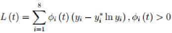
In this section, we apply the Lyapunov method and the LaSalle’s Invariant principle to prove the global stability of the endemic equilibrium point (EEP) of the model system (1). Now, consider a continuous and differentiable Lyapunov function defined as;

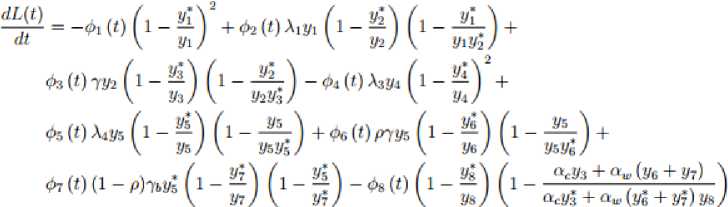
Where ф ( t ) is a positive constant factor, y_t is the i t variable at compartment i and y_t is the equilibrium point of the model at compartment i where i = (1,2,...,8). Differentiating L ( t ) w. r . t and substituting the constants of the model system (1) at the endemic equilibrium point into the function (23) we get;

t hus from equation (24) we have,

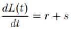
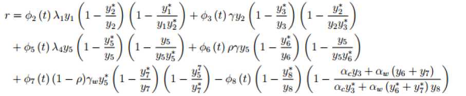
where,

and

8 = ~Ф1 (t)(l--

\ У1

Using the theorem (4.2) and the equation (24), the global stability holds only if dLtl < g. Now if r < 5 dt then dL(t) will be negative definite which implies that dL(t) < q But dL(t) = gonly if yt = yt for i = 1,2, dt                                                             dt .         dt

...

,8.

J                   dL (t)_ 1

I y 1 , y 2 ,..., y 8 ^e^ •          ° Г

Hence the largest invariant set I                   dtis a singleton y . By the LaSalle’s invariant principle [12], it is then implies that y . is globally asymptotically stable in the invariant region if r < 5 and thus Ro > 1. We then establish the following Theorem;

Theorem 4.3 The Endemic Equilibrium Point Q * of a Newcastle disease transmission model (1) is globally asymptotically stable if R >  1.

• 5.    Results and Discussion

  In this section, numerical simulations of the mathematical model (1) are conducted to study the dynamics of ND in village chicken population in the absence of any intervention. For the simulation we use the value of R and other model parameter values as given in t able 2 . t he total population of village chicken and wild birds is assumed to be two thousand and five thousand respectively. Using the estimated parameter values given in t able 2 , we obtain the basic reproduction number, R_o = 0.5692732754 <  1 which by the theorem (4.2) the disease free equilibrium point Q ⁰ is locally asymptotically stable. However, with the values given in the Table

  2 and the estimated parameter value of φ = 0.003, α = 0.0002, ψ = 0.00083, and a = 0.0003 we obtain R = 6.867182099 >  1 at the endemic equilibrium point and by the theorem (4.3) , it follows that endemic equilibrium point Q ^* = { S ^* , E ^* , I ^* , S ^* , E ^* , I ^* , I ^* , H } exists and is globally asymptotically stable.

• 5.1.    Variations of Population Variables on the Dynamics of ND Over Time

Table 2. Parameter Values of the Model System 1

Parameter	Parameter value	Source
γ	0.067 – 0 . 5 day - 1	[1, 8, 20]
φ	0.003 day - 1	Estimated
b	0.21 day - 1	[1, 8]
α c	0.001667 day - 1	Estimated
α w	0.00002 day - 1	Estimated
ψ	0.00083 day - 1	Estimated
µ	2.74 – 5.48 × 10 - 4 day - 1	[14]
a	0.003 day - 1	Estimated
δ c	0.01989 day - 1	[9]
ρ	0.9	Estimated
d	0.001 day - 1	[6]
δ w	0.025 day - 1	[7]
µ v	0.00219 day - 1	[7]
k	10000 virus / m - 3	[6]

d ifferent initial values and the given parameter values in t able 2 are used to illustrate numerical stability of the disease free equilibrium point Q ⁰ and the endemic equilibrium point Q * of the NDV transmission model system given in (1). 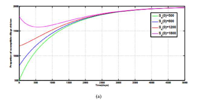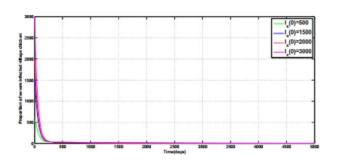With different initial values for S ( t ) , S ( t ), I ( t ) and H ( t ), the curves for the severely infected village chicken I ( t ) converges to zero along the time axis whilst susceptible population curves of the village chicken S ( t ) converges to a unique point as shown in Fig .1 (a) and Fig.1 (b). This reveals that the disease free equilibrium point Q ⁰ exists and is Stable for R < 1.

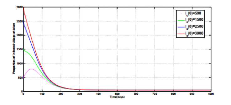
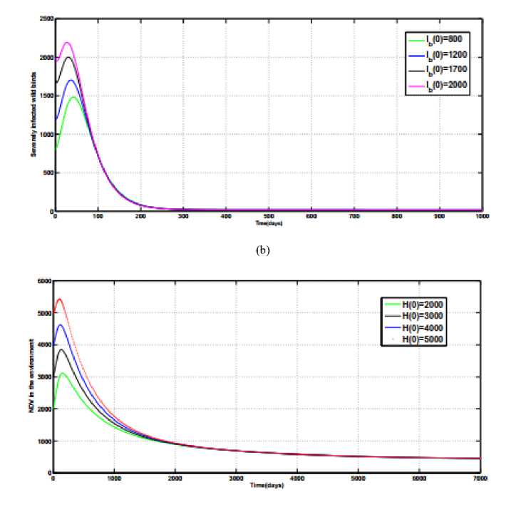
Fig.2(a), Fig.2(b) and Fig.2(c) illustrates the numerical simulations for the endemic equilibrium point of the model (1). Starting with different initial values and using the parameter values given in Table 1 and φ = 0.003 , α = 0.0002, ψ = 0.00083 and a = 0.0003 for R >  1, the state variables I ( t ), I ( t ), and H ( t ), populations curves converges to the unique points above zero. The results of these figures prove that for R >  1 the endemic equilibrium point Q ⁰ , of the model system (1) exists and is stable.

(b)

Fig.1. Stability of the Disease Free Equilibrium Point, (DFEP) using the Parameter Values Given for R <  1.

(a)

(c)

Fig.2. Stability of endemic equilibrium point, ( Q *) of the model system (1) using parameter values given in table for R >  1.

• 6.    Conclusion

In this paper, we presented the stability analysis of the equilibrium points of the basic transmission model of ND for the free-range managed chicken without any control as developed by [6]. The model has two equilibria points, the disease free equilibrium point and the endemic equilibrium. The local stability of disease free equilibrium point is done analytically by using the Hurwitz Matrix method and we establish a theorem that under some given conditions the disease free equilibrium point is locally asymptotically stable. Using numerical simulations we confirmed that the disease free equilibrium point is locally asymptotically stable for Ro < 1.and the infected compartments converges to zero, while the susceptible compartment converges to a unique point above zero. Furthermore, we presented the analysis for the stability of the endemic equilibrium point of the model using the Lyapunov function and the Laselle’s theorem. The analysis shows that the endemic equilibrium point is globally asymptotically stable when Ro > 1. The existence of endemic equilibrium point was further confirmed numerically that regardless of the values of the initial condition of the state variables, the infected compartments converges to a unique point above zero which shows the persistent of disease in the population. Thus, the analysis presented in this paper shows that the transmission model for the ND among the village chicken population with the vital component of contaminated environment and wild birds is epidemiologically meaningful.

This work provides an insight for looking different control strategies that considers the main agents in the dynamics of the ND. The controls will be helpful for the village chicken keepers in reducing the seasonal and periodic occurrence of the disease among village chicken population.

Acknowledgment

The authors would like to thank the Dar es salaam University College of Education (DUCE) for material support.

Conflict of Interests

No conflict of interests declared by author.