Statistical analysis of operational reliability of hydraulic structures

Author: Rustamov Yasin Ismail, Hasanov Sabir Tehrankhan
Journal: Природные системы и ресурсы @ns-jvolsu
Section: География и геоинформатика
Article in issue: 3 т.7, 2017.
Free access
In the paper, according to actual operation of pump units it was determined that operattion period of to their failure corresponds to Weibull distribution. In periods between failures, conditionally the pump units were considered as unrepairable. Therefore, not the availability factor and operation period between failures that are the complex reliability indices characterizing reliability of a pump station but probability of continuous operation and mean value of continuous operation time were calculated. The role of continuously loaded resource in reliability increase of the system was determined. The report was executed by the mathematical software program package “Derive - 6”.
Pump unit, continuity, reliability, quality (failure), criterion, probability, random events, structural design
Short address: https://sciup.org/149131430
IDR: 149131430 | UDC: 504:626 | DOI: 10.15688/jvolsu11.2017.3.7
Статистический анализ эксплуатационной надежности гидротехнических сооружений
В статье, согласно фактическим периодам работы насосных агрегатов, было определено, что времени их работы до отказа соответствует распределению Weibull. В периоды между отказами насосные агрегаты условно рассмотрены как невосстанавливаемые. Поэтому вычислено вероятность безотказный работы и средняя наработка до отказа, а не коэффициент готовности и периоды работы между отказами, которые являются сложными комплексными показателями надежности, характеризующими надежность насосных станций. Была определена роль постоянно нагруженного резерва в увеличении надежности системы. Расчет был выполнен пакетом математической программы «Derive-6».
Text of the scientific article Statistical analysis of operational reliability of hydraulic structures
DOI:
evacuated from irragation and water services by the existing pump stations is 5 billion cubic maters per year including, 2 billion cubic meter collectordrainage waters [1]. Provision of continuity of water evacuation and the required pressure in water management system is mainly determined by
In Azerbaijan, over different purpose 1000 pump stations are being operated. They are mainly used for water transport from water reservoirs to certain distances, evacuate collector-drainage waters from sown areas. Total amount of water reliability of pump stations. Lower reliability pumping stations increases operating costs, reduces service life and economic efficiency. At the same time, failure of low efficiency pump stations leads to great material and financial losses [2, 3].
Failure of normal operation of pump station during operation time is connected with random events. For evaluating no-failure operation of a pump station its probability character reliability indices should be known. A number of precious and complex characteristics are among these indices. Precious reliability of pump stations contain their no-failure operation probability P(t) and mean operation time T0to failure. The availability factor Kh and operation periods T between failures belong to complex reliability indices that characterize nofailure operation and repairability of a pump station [4, 5]. According to normative requirements when evaluating the reliability of restored equipments it is required to calculate Kh and T0. In interrepair period the pumps may be conditionally considered as unrepairable equipments. Therefore, in these equipments the avaibility factor coincides with continuous operation probability or has the same sense [6].
Problem statement
The object of this research is “Shimal-2” pump station in Salyan region of Azerbaijan. The pump station consists of three pumping units (two
16 NDN and one 24 NDN) and is used for meliorative purposes.
Operation hours of the pump station on the period of one year is given (table 1).
As a zero hypothesis we assume that variation series ( t, n t2 n .... n t r ) 5 = 0 of operation hours of pumping units is subjected to two-parameter Weibull distribution law. If the zeroth hypothesis is rejected, then other distributions, including three-parameter Weilbull distribution may be considered. Mann and other authors have used only goodness of first criterion prepared for Weibull distribution [7, 8, 9].
Problem solution:
Table 2 was drawn up for finding the values of observation criterion for the first pump unit.
By goodness of fit criterion, S m » 0 ,29 .
Using special tables, according to accuracy level r = 10 and a = 0,05 it was determined that the critical value of the criterion is S b = 0 ,69 . As S m n S b , in this case, it was determined that the operation hours between failures corresponds to two-parameter Weibull distribution, and the distribution function
-
- (-)Ь
F (x ;a,b ) = 1 - e a x - 0 (1)
here a is the scale or resource parameter, b is the shape parameter or angular coefficient.
Table 1
Actual operation hours of “Shimal -2” pump station
|
№ of PU |
On months |
Type of the pump |
||||||||||
|
I |
ІІ |
ІІІ |
ІV |
V |
VІ |
VІІ |
VІІІ |
ІX |
X |
XІ |
||
|
1 |
248 |
252 |
351 |
450 |
480 |
440 |
445 |
362 |
390 |
415 |
- |
16NDN |
|
2 |
350 |
357 |
463 |
514 |
512 |
521 |
585 |
396 |
275 |
312 |
425 |
16NDN |
|
3 |
196 |
340 |
270 |
310 |
335 |
364 |
200 |
273 |
445 |
300 |
285 |
24NDN |
Table 2
Operation hours of the first pumping unit
|
i |
t i |
x i = lnt i |
Mi |
x i + 1 - xi |
(xi + 1 - xi) / Mi |
|
1 |
248 |
5,5134 |
1,054 |
0,016 |
0,0152 |
|
2 |
252 |
5,5294 |
0,559 |
0,3314 |
0,5928 |
|
3 |
351 |
5,8608 |
0,399 |
0,0308 |
0,0772 |
|
4 |
362 |
5,8916 |
0,325 |
0,0745 |
0,2292 |
|
5 |
390 |
5,9661 |
0,286 |
0,0622 |
0,2175 |
|
6 |
415 |
6,0283 |
0,269 |
0,0585 |
0,2175 |
|
7 |
440 |
6,0868 |
0,271 |
0,0113 |
0,0417 |
|
8 |
445 |
6,0981 |
0,301 |
0,0111 |
0,0369 |
|
9 |
450 |
6,1092 |
0,405 |
0,0646 |
0,1595 |
|
10 |
480 |
6,1738 |
If we make the substitution x = Int , then distribution function of the random variable x is
Here a i and c i are linear weighted multipliers. Initial parameters and reliability of the Weibull distribution is calculated as
F (x ) = 1 - exp[ - exp(-----)]
v
( —да п x п да ) (2)
here u = Ina and v = — . When the reliability ( P ) of the equipment is known, for finding the random variable x, we can write expression (2) as follows:
|
a = eu , |
(6) |
|
ь = 4 , v P(t) = exp ( - -)b |
(7) |
|
(8) |
a
x = U + v [ln(ln—)] (3)
Linear weighted sets found for r = 10 from special tables are given in table 3.
By making the substitution xi = lnti the coefficients in expression (3) are calculated as u =ТЛ ■ xi, (4)
i = 1
v h c ■ x i . (5)
I = 1
and is called the best unchangeoble linear assessment. This assessment gives the least error with regard to other assessments. From the expressions (5) and (6), as u = 5,6092 , v = 0,1571 in expression (7) and (8) hours a = 273 , b = 6,36 . Then from dependence (9) in the general form we get
Pi() = exp( - -)b = exp( - -^—,>3,36 . (9) a 273
Expression (10) represents no-failure operation probability of the first pumping unit. Table 4 was drawn up for determining regularity of distribution of non-failure operation time of the second pumping unit.
Table 3
|
t i |
x i = lnt i |
a i |
c i |
|
248 |
5,5134 |
0,0273 |
-0,07273 |
|
252 |
5,5294 |
0,0400 |
-0,07797 |
|
351 |
5,8608 |
0,0525 |
-0,07724 |
|
362 |
5,8916 |
0,0654 |
-0,07188 |
|
390 |
5,9661 |
0,0793 |
-0,06165 |
|
415 |
6,0283 |
0,0946 |
-0,04542 |
|
440 |
6,0868 |
0,0946 |
-0,02070 |
|
445 |
6,0981 |
0,1124 |
0,01793 |
|
450 |
6,1092 |
0,1342 |
0,08507 |
|
480 |
6,1738 |
0,2300 |
0,32460 |
Table 4
Operation hourse of the second pumping unit
|
i |
t i |
x i = lnt i |
Mi |
xi + 1 - x i |
(xi + 1 - xi) / M i |
|
1 |
275 |
5,6168 |
1,0484 |
0,1262 |
0,1204 |
|
2 |
312 |
5,7430 |
0,5528 |
0,1141 |
0,2064 |
|
3 |
350 |
5,8579 |
0,3914 |
0,0198 |
0,0506 |
|
4 |
357 |
5,8777 |
0,3147 |
0,1037 |
0,3295 |
|
5 |
396 |
5,9814 |
0,2732 |
0,0707 |
0,2588 |
|
6 |
425 |
6,0521 |
0,2514 |
0,0856 |
0,3405 |
|
7 |
463 |
6,1377 |
0,2439 |
0,1006 |
0,4125 |
|
8 |
512 |
6,2383 |
0,2515 |
0,0039 |
0,0155 |
|
9 |
514 |
6,2422 |
0,2839 |
0,0153 |
0,0539 |
|
10 |
521 |
6,2575 |
0,3891 |
0,1141 |
0,2859 |
|
11 |
585 |
6,3716 |
By the expression of the goodness of fit criterion, Sm = 0,53 . By the number of failures r = 11 and accuracy level a = 0,05 it was determined from special tables that Sb = 0,74 . As S m n S b , distribution of no-failure operation time of the second pumping unit mets the Weibull distribution.
Table 5 was drawn up to determine no-failure operation probability of the Weibull distribution parameters and the second pumping unit.
As in dependence (5) and (6) we get u = 6,5196 , v = 2,1247 , from expressions (7) and (8) a = 678 hours , b = 0,47 . In this case for the second pumping unit formula (9) must be calculated as follows
P 2(t) = exp ( - T t-) 0’47 . (10) 678
Table 6 was drawn up to determine regularity of distribution of no-failure operation time of the third pumping unit.
If we take into account the values in Table 6 in the expression for the goodness of fit criterion, then S m - 0,54. By the number of failures ( r = 11 ) and from the accuracy level ( a = 0,05 ) from special tables S b = 0,74 . As S m n Sb , distribution of no-failure operation time of the third pumping unit meets the Weibull distribution.
For finding no-failure operatrion probability of the third pumping unit, at first the parameters should be determined. To this end, table 7 was drawn up.
Table 5
|
t i |
x i = lnt i |
a i |
c i |
|
275 |
5,037 |
0,016 |
-0,070 |
|
312 |
5,347 |
0,034 |
-0,074 |
|
350 |
5,375 |
0,043 |
-0,074 |
|
357 |
5,481 |
0,054 |
-0,071 |
|
396 |
5,846 |
0,066 |
-0,064 |
|
425 |
6,040 |
0,078 |
-0,054 |
|
463 |
6,047 |
0,093 |
-0,039 |
|
512 |
6,174 |
0,111 |
-0,019 |
|
514 |
6,242 |
0,133 |
0,010 |
|
521 |
6,256 |
0,347 |
0,052 |
|
585 |
6,372 |
0,098 |
0,402 |
Table 6
Operation hours of the third pumping unit
|
i |
t i |
x i = lnt i |
Mi |
xi + 1 - xi |
(xi + 1 - xi ) / M i |
|
1 |
196 |
5,2781 |
1,0484 |
0,0202 |
0,0193 |
|
2 |
200 |
5,2983 |
0,5527 |
0,3001 |
0,5430 |
|
3 |
270 |
5,5984 |
0,3914 |
0,087 |
0,2223 |
|
4 |
273 |
5,6095 |
0,3147 |
0,043 |
0,1366 |
|
5 |
285 |
5,6525 |
0,2732 |
0,0513 |
0,1878 |
|
6 |
300 |
5,7038 |
0,2514 |
0,0328 |
0,1305 |
|
7 |
310 |
5,7366 |
0,2439 |
0,0775 |
0,3178 |
|
8 |
335 |
5,8141 |
0,2516 |
0,0149 |
0,0592 |
|
9 |
340 |
5,8290 |
0,2839 |
0,0682 |
0,2402 |
|
10 |
364 |
5,8972 |
0,3807 |
0,2009 |
0,5277 |
|
11 |
445 |
6,0981 |
Table 7
|
ti |
x i = lnt i |
a i |
c i |
|
196 |
5,2781 |
0,0249 |
-0,0654 |
|
200 |
5,2983 |
0,0355 |
-0,0703 |
|
270 |
5,5984 |
0,0457 |
-0,0705 |
|
273 |
5,6095 |
0,0562 |
-0,0671 |
|
285 |
5,6525 |
0,0673 |
-0,0602 |
|
300 |
5,7038 |
0,0792 |
-0,0493 |
|
310 |
5,7366 |
0,0926 |
-0,0332 |
|
335 |
5,8141 |
0,1080 |
-0,0094 |
|
340 |
5,8290 |
0,1271 |
0,0269 |
|
364 |
5,8972 |
0,1532 |
0,0891 |
|
445 |
6,0981 |
0,2104 |
0,3094 |
In the similar way, as from dependences (7) and (8) u = 5,8092 , v = 0,2066 from expressions (9) and (10) we get the values a = 334 hours, b = 4,8403 . In this case, for the third pumping unit expression (3) should be calculated as follows
P 3 (t) = exp( - 33 t 4 )4,84
Reliability and failure probability of the pump station are calculated as follows [4]
Pn / st = ∏ Pi , q ≈ 1 - P n / st ( t ) . (12)
i = 1
In the case of a reserved pump unit it is calculated as
P n / st = N ∑ - nC N i (1- P 0 ) i ⋅ P 0 N - 1, i = 0
q n , N = C N nP 0 N - n (1- P 0 ) n .
In expressions (11), (12), (13) and (14), giving different values to t , we can calculate reliability of pump units, in general of a pump station by formulas (15) and (16).
As is seen from the operating mode of a pump station, the system has a structural design with constant resource Fig. 1
λ 1
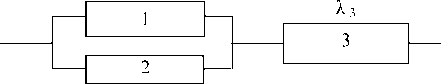
λ 2
Fig.1. Reliability block-design of the pump station
In such designs, the side-by-side connected element provides distribution or lowering of load.
The system’s reliability was calculated by the following expression:
P s ( t ) = [1 - (1 - e - ( t /273)6,36) ⋅ ⋅ (1 - e - ( t /678) 0.,47)] ⋅ e - ( t /334) 4,84 (14)
If we assess the functions on the interval 0 ^300 by 25 hour steps, we get the following table 8.
By integrating the expression (14) of probability of continuous operation of the pump station on the interval [0, ∞ ], we get that mean value of continuous operation time of the system [10, 11]
T = ∫ ∞ [1 - (1 - e - ( t /273)6,36) ⋅ (1 - e - ( t /678)0.,47)] ⋅
0 (15)
⋅ e - ( t /334) 4,84 dt = 273
is about 273 hours.
The graph of probability of continuous operation of pumping units and the pump station is depicted in fig. 2. The number of curves corresponds to numbers of pumping units. N/st is the graph of continuous operation probability of the system.
As is seen from the curves, the continuous operation probability of the system, in the case of distribution of operation time to failure by the Weibull law gets large values in small domains, gets small values at large values of t .
Failure probability of the system, density of distribution of continuous operation time to failure, and failure intensity of continuous operation time to failure are calculated as follows:
Table 8
|
ti hours |
P 1 (t) |
P 2 (t ) |
P 3 (t ) |
Pn/st(t) |
|
0 |
1 |
1 |
1 |
1 |
|
25 |
0,999 |
0,81 |
0,999 |
0,9999 |
|
50 |
0,999 |
0,75 |
0,999 |
0,9998 |
|
75 |
0,999 |
0,70 |
0,999 |
0,9991 |
|
100 |
0,998 |
0,67 |
0,997 |
0,9965 |
|
125 |
0,993 |
0,64 |
0,991 |
0,9889 |
|
150 |
0,978 |
0,61 |
0,979 |
0,9710 |
|
175 |
0,94 |
0,59 |
0,957 |
0,9345 |
|
200 |
0,87 |
0,57 |
0,920 |
0,8686 |
|
225 |
0,75 |
0,55 |
0,86 |
0,7645 |
|
250 |
0,57 |
0,54 |
0,78 |
0,6235 |
|
275 |
0,35 |
0,52 |
0,68 |
0,4658 |
|
300 |
0,16 |
0,51 |
0,55 |
0,3231 |
Q s = (1 - e - ( t /273)6,36 ) ⋅ (1 - e - ( t /678)0.,47 ) ⋅ (1 - e - ( t /334)4,84 ) (16)
fs ( t ) = ∂ ∂ t ((1 - e -( t /273)6.36 ) ⋅ (1 - e -( t /678)0.47 ) ⋅ (1 - e -( t /334)4.84 ))(17) ∂ ((1 - e -( t /273)6.36) ⋅ (1 - e -( t /678)0.47) ⋅ (1 - e -( t /334)4.34))
λs ( t ) = [1 - (1 - e -( t /273)6.36 ) ⋅ (1 - e -( t /678)0.47 )] ⋅ e -( t /334)4.84 (18)
The appropriate curves were drawn using expressions (17), (18).
Accordance of the pump station to normative requirements, became possible at the expense of the created resource unit. After about ten continuous operations, as engineering service and some routine repairs of pump units was possible, the pump station’s effective operation was provided.
Conclusion
“Shimal-2” pump station was designed without taking into account reliability conditions. In such cases, as the engineering equipment does not satisfy the reliability requirements, there occur failure cases, exploitation costs increases, continuous operation periods decrease and as a result, the equipment fails before ending the exploitation period or operates without some effect. In the paper, though the field of service of the pump station used for meliorative purposes and amount of water required for injection are
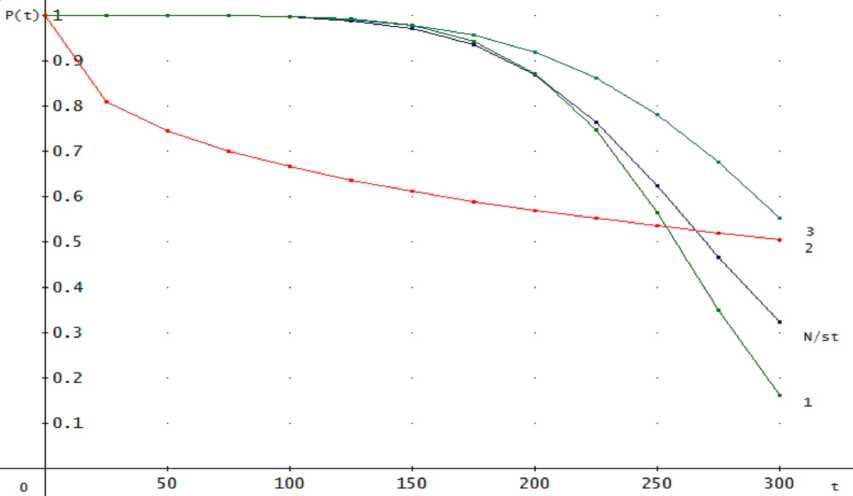
Fig. 2. Continuous operation probabilities of pumping units and pump stations
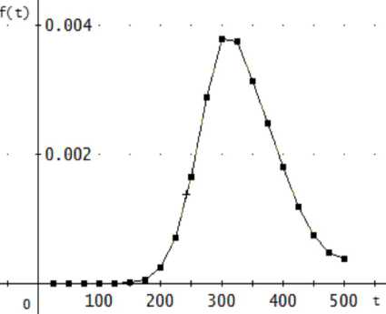
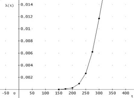
Fig. 3. Density of distribution of time to failure Fig. 4. Intensity of distribution of time to failure
not touched, it is known that according to operation hours, every unit works not by its total power but with itervals i.e. in the case when two pumps work with total power and another unit is in reserve, the system fulfiles its function i.e. the pump station has a permanently installed resource unit. According to theoreticcal results and graphical descriprion, “Shimal-2”, though the pump station is exploited for a long period, it was determined that this station meets the reliability requiremants.
In addition to other reasons, this was succeseded by permanently installed resource. In the paper, all three variants for determining the system’s reliability were used. They are structural design, operation hours and laow of distribution of continuous operation to failure.
In spite of such random cases, any engineering system must be designed, built and expoited with regard to reliability indices.
ПРИМЕЧА НИЕ
-
1 This work was supported by the Science Development Foundation under the President of the Republic of Azerbaijan-Grant № EЭF-KETPL-2-2015-1(25)-56/13/1.
References Statistical analysis of operational reliability of hydraulic structures
- Ahmedzade A.S., Hashimov A.S., Ensyclopedia on melioration. Baku, Radius, 2016, 632 p.
- Rustamov Y.I. Reliability conditions and reasons of failures in pump stations, Azerbaijan Agrar Elmi, vol. 3, 2013, pp. 111-114.
- Rustamov Y.I. Assessment of reliability of land-reclamation pump stations Investia Agrarnoy nauki, vol. 8, vol. 2, 2010, pp. 69-72.
- Polovko A.M., Gurov S. V. Bases of the theory of reliability. St. Petersburg, Petersburg, 2008, 702 p.
- Gnedenco B.V., Belyaev Y.K., Solovyov A.D. Mathematical methods in the theory of reliability. Moscow, LIBROKOM, 2013, 584 p.
