Stochastic Characterization of a MEMs based Inertial Navigation Sensor using Interval Methods

Published Online June 2015 in MECS DOI: 10.5815/ijigsp.2015.07.04

Process dynamics in conventional approach towards multi-sensor data fusion, are only known with some degree of certainty. The basic approach to handling this inconvenience has traditionally been to appeal to a probabilistic description of this uncertainty, via the inclusion of a process and a measurement noise, and apply a statistically optimal filter such as the Kalman Filter. This approach carries with it the necessity to introduce experimentally some distribution law describing the process and measurement noise. An alternative approach to treating processes with uncertain data is to apply the notions and methods of interval analysis. The idea of using interval arithmetic to describe the uncertainty in the system model was proposed in the late 90’s (Chen et al, 1997). This type of uncertainty can easily arise in practice. For example, when modelling from first principles, the values of certain physical parameters may not be known exactly, but known to lie within certain bounded limits with absolute certainty. Or when using system identification techniques to model a dynamic system, several models that differ only in the values of the matrix coefficients may be obtained under slightly different conditions, and these may all be contained in an interval.

Coming to sensor fusion, stochastic estimators are instrumental only in realizing covariance for overall estimation error. This is however significantly affected by the measurement error margin, which in the conventional approach remains unchanged throughout the entire estimation cycle. Interestingly the stationary measurement error margins fed into the estimation block initially are liable to evolve over time, due to unprecedented drifts encountered by the sensors. It is in this context that work is carried out in incorporating an interval based sensor fusion algorithm for an integrated navigational sensor suite. The algorithm is capable of determining dynamic error margins for a low cost MEMs based inertial navigation sensor on the one hand. At the other side the algorithm is shown to effectively reduce the error bounds for an integrated GPS, compass and Doppler velocity profiler meant for autonomous navigation of unmanned marine vehicles.

As regards navigation measure for autonomous marine vehicles, use of commercially available low cost MEMs inertial navigation sensors has grown into a recent trend. Although their suitability for short range operations is very obvious due to their high levels of drift, the cost effectiveness gives way for integration of other navigation aids. Extensive work has been put into studies of errors commonly associated with such systems. Various calibration and stochastic modelling methods have been proposed in this regard. However most of the proposed methods aim only at the stationary characteristic of such errors, with little attention towards dynamic drifts.

The two distinct types of error sources to be considered for MEMs inertial sensors are deterministic and stochastic. Fig. 1 illustrates a categorization of typical errors associated with inertial navigation sensor. The former relates to systematic errors emanating due to physical processes like mechanical misalignments, bias and scale factor. The latter however relate to the random fluctuations depending upon stochastic variations of errors over definite periods of time. While the former can be resolved through standard calibration measures, the latter is very difficult to completely eliminate and hence need to be modelled using statistical processes. A detailed description of such errors is provided in [1]. In the present context, we shall restrict the discussion to the stochastic modelling of errors associated with measurements of low cost MEMs inertial sensor.

Deterministic/

Systematic

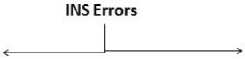
Bias

Instability

Drift Rate Ramp

Bias

Scale Factor

Misalignment /

Non orthogonality

Stochastic

Random Walk

Scale factor stability / Repeatability

Angle          Velocity

Random Walk Random Walk

Fig.1. Classification of errors typically associated with measurements from Inertial Navigation Sensors

Reportedly Autocorrelation Function has been primarily used for stochastic modeling of inertial sensor errors. Autocorrelation function determines the dependence of data values of stationary process at one time on values recorded at another time. However accuracy of estimating parameters for the autocorrelation process depends upon length of static data recorded from the sensor. In view of this fact, another robust stochastic modeling technique defined as Autoregressive process has been adopted. Autoregressive processes have greater modeling flexibility since they are not always restricted to only one or two parameters. The model parameters for such process can be effectively computed by solving a set of linear equations. The work of Nassar [2], Noureldin et al [3] reflects use of autoregressive processes as modeling tool for stochastic error analysis of inertial sensor. Noise is segregated into short-term as well as long-term errors. Short term random errors have been modelled using fist ordered Gauss Markov process, defined as follows:

xt+δt =(I- βδt)xt +  2βσ2ωt+δtδt

Where X (_t+5_t) is the current observation, в being the reciprocal of correlation time, ro (_t+g_t) is the white noise having density у and St is the sampling time. On the other side a p -th order polynomial fitting is done for realizing long term correlated errors using autoregressive process. Burg estimation method [4]-[6] is used for determining the parameters of the AR model defining the sequence in time-domain as follows:

p

The Burg method is used to fit a p -th ordered AR model to the input signal by minimizing the forward and backward prediction errors.

Interestingly however, variance analysis methods have been widely used for studies of static errors associated with inertial sensors. Most important of such methods is the Allan Variance technique of determining critical noise coefficients for stochastic errors. The seminal work of David Allan [7] in computing correlation co-efficient simply through a time averaged procedure has been subsequently put to error analysis of inertial sensors profoundly in the thesis work of Haiying Hou [8], Park [9] and Naser et al [10]. Allan variance is a method of representing root mean square (RMS) random drift error as a function of averaged time. Consequently, Allan variance method is incorporated to determine the characteristics of the underlying random processes that give rise to data noise. The data is normally plotted as the square root of the Allan variance versus T on a log-log plot.

In the present scope of work, Allan Variance method is used at the first hand, in order to characterize a low cost MEMs sensor by recording static data over a significantly long period of time. Subsequently, static noise coefficients are computed using cluster time averaged variance analysis. At the second phase, dynamic errors are estimated using interval analysis over data collected from an integrated sensor framework consisting of the inertial sensor, a compass and a GPS receiver. The dynamic error margins are computed using interval contractions.

• II. Background

• A.    Stochastic Analysis of Stationary Errors

Allan variance analysis is carried out to realize two dominant noise terms associated with stationary data viz. random walk and bias instability parameters. A short description, as to how to compute the non-overlapping Allan variance out of stationary data, is being presented.

Assume that there are N consecutive data points, each having a sample time of t 0 . Forming a group of n consecutive data points (with n < N/ 2), each member of the group is a cluster. Associated with each cluster is a time T , which is equal to nt 0 . If the instantaneous output rate of the inertial sensor is Ω ( t ), the cluster average is defined as:

t_k + T

T t k

Where, represents the cluster average of the output rate for a cluster which starts from the k-th data point and contains the n data points. The definition of the subsequent cluster average is tk+1 +T tk+1

Where t (k+1) =t k +T

Performing the average operation for each of the two adjacent clusters can form the difference

ξ = Ω (T) - Ω (T)

k + 1, k       next            k

For each cluster time T, the ensemble of ξs forms a set of random variables. The quantity of interest is the variance of ξs over all the clusters of the same size that can be formed from the entire data. Thus, the Allan variance of length T is defined as [11]:

N - 2 n

σ ² ( T ) = ¹ ∑ [ Ω next ( T ) - Ω k ( T )] ² 2( N - 2 n ) k = 1

In order to carry out the necessary exercise on stochastic modeling a low cost MEMs inertial sensor Mtx of Xsens make has been employed. The specifications of the sensor are as tabulated in Table.1. The Allan deviation plots for accelerations and angular rate are shown in Fig. 2.

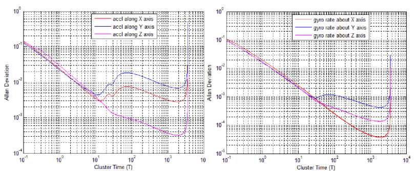
Fig.2. Plot for Allan Deviations against acceleration (left) and gyroscope (right) measurements during static tests with Mtx INS

Data from the Mtx inertial sensor was recorded over an uninterrupted duration of 2 hours, and the stochastic variations in the observed errors were studied in order to compute the random walk and bias instability co-efficient. Angle (/Velocity) Random Walk is denoted by N . The error grows as N x √sec, and is modelled as white noise. On the other hand, Bias Instability is denoted by B, and defined as a random variable variance of which grows over time in correlated manner. It is usually modelled as a first-ordered Gauss Markov noise variable. The random walk and bias instability coefficients are provided in Table 1 as follows.

Table1. Specifications for Mtx inertial navigation sensor from Xsens

Type of Sensor	Physical Type	Bias Stability (1-sigma)	Alignm ent Error	Noise Density
Accelerome ter	MEMs solid state, capacitativ e readout	0.02m/sec2	0.10	0.002 m/sec2/√H z
Rate Gyroscope	MEMs solid state, beam structure monolithic , capacitativ e readout	10/sec	0.10	0.05 deg/s/√Hz

The cumulative effect of both the above-defined types of errors may be consolidated into a single white noise representative standard deviation as follows:

σ _c

N

δ _ttB

Consequently, the intervals for accelerations and angular rates can be drawn out as follows:

• B.    Stochastic Analysis of Dynamic Errors

In the present scope of work interval method is used in analyzing dynamic uncertainties for a low cost MEMs inertial sensor. The present work has been carried out with an integrated sensor suite consisting of a GPS, a compass along with an inertial motion unit. Error bounds for all the sensors have been translated into guaranteed intervals. GPS based position intervals are fed into a forward-backward propagation method in order to estimate interval valued inertial data. Dynamic noise margins are finally computed from comparisons between the estimated and measured inertial quantities. It is therefore meaningful in constraining errors from individual measurements so that the estimated data (position in the present context) may well be defined within guaranteed intervals. Stochastic models involving few probabilistic approximations are not complete representation of the true characteristic of errors, whereas intervals can be more reliable, in a sense that they tend to typically restrict the boundaries for maximum drift and that they can provide for a worst case performance analysis of any sensor fusion algorithm.

• C.    Error bounds for Compass and GPS receiver

Error in compass measurements arises from imperfect calibration or the presence of some additional magnetic field in the calibration area or at the field site. Compass error is therefore typically a function of the measured heading. Because the origin of this compass error is due to external magnetic forces, the error is well represented by a one-cycle (hard iron) model [12]:

Where ψ err is the total error in heading, ψ is the measured heading, A , B and C are obtained from calibrating the compass with reference to some magnetic needle. Subsequently, the non-punctual heading can be constructed as:

I V 1= [V-Verr ,V + Verr ]

However, position fixes from GPSs suffer from different types of noise associations [13] which may either be associated with the loss of sync between satellite (SV) and receiver atomic clocks, or due to paucity of proper SV geometry. The latter phenomenon dilutes a position fix to a great extent even with limited noise in range measurements, as obtained by the receiver from the available satellites. The performance index for any GPS is defined in terms of dilutions of precision (DOP) [14] categorized as position (PDOP), vertical (VDOD) and horizontal (HDOP). The HDOP is accepted more popularly as a measure of accuracy for the twodimensional planar position of the receiver. It is numerically defined as:

HDOP = ^v __ y

^ R

Where σx and σy are the standard deviations for X and Y coordinates with σR termed as User Equivalent Range Error (UERE). Since HDOP is highly affected by the satellite geometry, the GPS measurements may suffer from varying HDOP measures with the same margin of noise in range measurement. However, low HDOP measure for a given fix evidently means greater position accuracy. Considering a HDOP measure of unity there are other common definitions of accuracy of a GPS position fix. Circle of Equi-Probable error (CEP) is another common performance measure, usually provided by GPS manufacturers. The distance specified as CEP for a given GPS means that the actual position of the receiver remains with 50% probability within a circle centered at the measured position and having as radius the distance specified as CEP. In more general terms the probability P of actual position, being within a specified radius of error D, is defined by using a Rayleigh distribution as follows:

Г D

Where the root mean square distance, DRMS is defined as √(σx²+σy² ) (Refer to [15]). Referring back to CEP error, we can find out the DRMS through a sequence of derivations as follows:

CEP

DRMS = z D

P(error < CEPd ) = 0.5

_( CEPd Y

I DRMS J

^ 1 - exp

CEP

^ DRMS = ln2

---Г

^ U_x ² + e r 2 =  _z D = 1.201

• x     y      ln2

A 95% confidence interval for positional error D is accordingly expressed as. However, considering a HDOP of unity the DRMS is the same as UERE. UERE being independent of the DRMS, in the case when motion of the vehicle is such that the view of the satellite geometry changes with a consistent UERE, DRMS is simplistically defined as:

HDOP x UERE _{( HDOP = l)} ^ DRMS ( i ) = HDOP(i ) x DRMS _{( HDOP = l)}

Where, ‘ i’ is the sampling instant. Finally the mean GPS error μ e can be defined as follows:

M e = ^ DRMS ( i ) = ^ HDOP ( i ) x DRMS ₍ hdop =„

The non-punctual position based on GPS observations may be expressed as:

• III.    Proposed Interval Based Algorithm

A little background on interval contractions is presented before deriving the equations in the present context. The FBP contractor is simplest among all contractors and works on the principle of primitive functions [16]. It consists of two steps, the first being propagating the dependent variables using the general form of equations. This results in updated intervals for the dependent variables. Subsequently, the second stage involves propagating independent variables using inverse functions, which results in contracted bounds. The cycle is repeated until no variable has a contracted interval. The process ultimately generates optimal contraction for the interval values associate with the variables. This may be illustrated with a simple example before defining the process in the context of sensor error interval fusion.

Let us consider a simple addition of two interval valued variables [x] and [y] which leads to a third variable [z]. Then the FPB contractor works as follows:

Forward Propagation :

[z]=[z] MM+[y] }

Backward Propagation:

[x]=[x] ^ {[z]-[y] }[y]=[y] n {[z]-[x] }

The FPB contractor is further used in Waltz algorithm [17] which involves repeated propagations back and forth until the intervals do not contract any more. However, in context of the present problem, the propagations are carried out once in order to ensure completion of the contraction process within a single sampling time. Moreover, the present application does not demand very sharp bounds for a worst case analysis of dynamic error margins associated with inertial measurements.

In the present scope of work the mechanization equations for inertial sensor are used for propagating intervals in the forward direction. Subsequently, GPS based equations are used for shrinking the intervals along a backward traversal. For the purpose of exploiting error intervals, positions have been expressed in the form of boxes as follows:

X

source

Psource

Psource

^{1 P}source । t +8 t   ^{{| P}source ^{( X} ) । t +8 t , ^{I P}source ⁽ y ) । t +8 t ^}

Where source represents the particular sensor from where data is obtained. In our case there shall be only two sources viz. GPS and INS. The forward set of mechanization equations are expressed with respect to a local East North Up {ENU (n-) [18]} navigation frame of reference. The body frame velocities are transformed into the reference frame and positions in the navigation frame are dead reckoned as follows:

I P NS ⁽ x ) I t +8 t =1 ^P NS ⁽ x ) I t ⁺ I u I t +8 t cos(I V 1 t +8 , )^{W —} | V | , sin| V 1 t ) &

1 ^P NS ⁽ У ) 1 t +8 t =1 P NS ⁽ У ) 1 t ⁺ I ^V 1 t +8 t ^COS(I V 1 t + 8 t ^{) 8t +} I ^U 1 t +8 t NI V 1 t +8 t ⁸

Where the interval based linear and angular velocities are computed as follows:

I u I

LI ^V U t +8t

I uI

_ I V I J t

+

I-I

I V I _л

Ы   U t+8t

8t

Hence GPS based positions may be computed in the navigation frame in order to carry out the backward set if equations. Relative positions with respect to the origin of the navigation frame are obtained through transformation of GPS coordinates as follows:

Where, S and represent the great circle distance and bearing between a pair of GPS coordinate, i.e. latitude and longitude. Distance and bearing are computed using Haversine formula as follows:

S = R x B

.  , ( C )

a = tanh l — I

I D )

Where the parameters A, B, C, D and R are defined as below:

I A )

C = cos la ( t )sin la ( t + 8 t ) — sin la ( t )cos la ( t + 8 t )cos A lo

R is the mean radius of Earth. Coming to the backward phase of interval contractions we are interested in formulating equations which shall represent non-punctual accelerations and angular rates. The difference in intervals between contracted ones and those predicted during the forward phase, may be considered as the dynamic error margins. Backward propagation of errors is formulated as follows:

ˆ

^{I X I} = ^XINS ¹ 1 +8 t ^ ^I X GPS ¹ 1 +8 t

IUI1+а=

co ^s(I V ¹ t +8 t ) . ^si n ^(I V ¹ t +8 . )

~

IU ,+8 = (U|t„ -[«I Ml)/8 I П,+8t=V„Н»1t)/8t

• 1.    Obtain acceleration and angular rate measurements U and r from INS.

• 2.    Compute intervals for acceleration and angular rate observations by considering noise margins as obtained from stationary characteristics

• 3.    Use forward propagation equations to obtain interval estimates for position as follows:

Where the velocity estimate in the navigation reference frame is denoted as X    and is expressed in the body fixed frame as U       Finally, non-punctual accelerations expressed in body frame and estimated from an inverse transformation of GPS interval position coordinates are expressed in the body-fixed frame of reference as U     Similarly, angular rate intervals are estimated from residual between current observation from compass and heading prediction in the previous sampling instant:

I rIt+HVU-IVl) / a

Where the estimated heading intervals are obtained as:

^{I V I} t +8 =^{V 1} 1 +8 ^П1 V c ¹ 1 +8

The latter representing intervals of compass heading defined with the error bounds of compass as:

^ c ¹ 1 +8 = [ ⁽ V c . +_a -V err )> Vc , 8_a ^ /Te ) ] ^)]

(^I x ^|,| y 0= 0 x ^|,| y D G ^u x ^{|,| y} D ^{8 t} + ¹ (^I x ^{|,| y} D ^8t2

^{I V >} H V ^I c ⁿ ( ^{V I + 1} r ^{I 8 t} }

Where, ( I x I,I y I )_G is the interval bounded GPS observation and the latter in intersection comes from kinematic model using INS data bounds. Similarly, I V Ic is the bounded Compass readout and the latter in intersection are the model predicted heading bounds

4. Use backward propagation equations to obtain estimated bounds for acceleration and angular rate as follows:

(I x I,I y I) = (I x I,I y I) n {(I x I,I y I) t +8 t - (I x I,I y I) t }/ 8t

^I r = ^{r I n {(I} V ¹ 1 +8 t ^{- 1} V ¹ 1 )/ ^{8 t }}

The obtained acceleration estimates can be transformed into body-fixed frame using the direction cosine matrix as stated previously.

The method discussed so far can be drawn into an algorithmic structure described in the following steps:

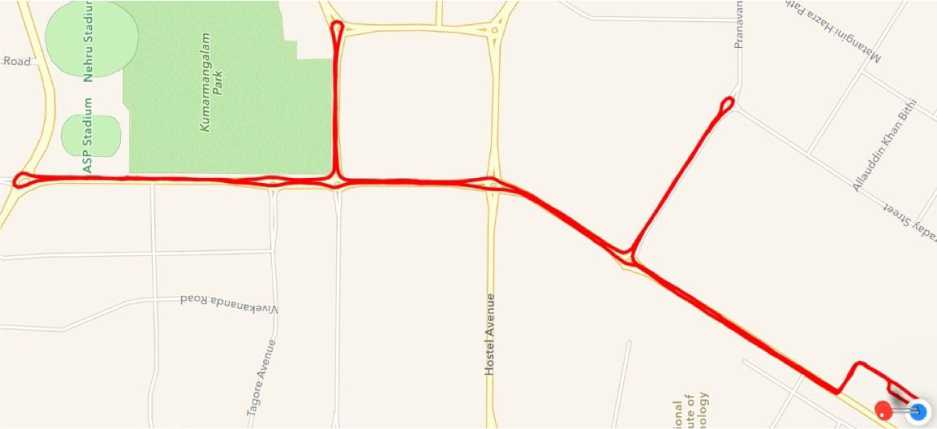
Fig.3. Position of the vehicle as tracked by GPRS based navigation tool on mobile handset

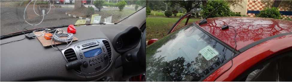
Fig.4. Placement of sensors on board the vehicle used for carrying out experiment. A platter is shown to be fixed on the dashboard (left) with Xsens INS and compass mounted on it. The GPS receiver is mounted on top of the roof for better signal reception.

• IV.    Experimental Validation and result analysis

  A MEMs inertial sensor of make Xsens has been used along with a GPS receiver from Rhydolabz and compass OS5000 from Ocean Server, all of which were mounted on a ground vehicle. Relative positions for the different sensors mounted on a car are depicted in Fig. 3. Compass and inertial sensor are mounted on a platter fixed with the vehicle and aligned with the vehicle's heading. The experiment involved a single closed trip covering a total distance of 9.4 kms with an average speed of less than 50 km/hr and over duration of 792 seconds, map of which is shown in Fig. 4. Medium quality GPS corrections were obtained with an average horizontal dilution of precision (HDOP) measure of < 0.8 and a circular error probability (CEP) of 3m. The GPS used for the said test platform suffers from a CEP error of 3 meters, which gives an approximated measure of DRMS as 3.6 meters. With a mean HDOP measure of 0.8 (as has been recorded over the entire duration of tests), the mean error in position is found to be 3.19 meters. Intervals for GPS obtained position measures are finally construed on the basis of the mean error, and are used subsequently.

0.2 m/sec2 for acceleration values along X and Y axes respectively.

Set of data collected from the above-mentioned three sensors was logged with a unique time-stamp, so that offline processing could be done effectively, with samples collected at a rate of 1 Hz.

In order to realize the effectiveness of the interval approach in assessing the dynamic noise margins associated with the inertial sensor, we need to revisit the static noise levels computed using variance method. The physical interpretation of Random Walk (RW) and Bias Instability (BI) coefficients may be discussed in the present context. RW introduces a stochastic error as a result of integrating a noisy signal whereas BI is the time averaged drift in bias associated with the original signal. RW has got a lesser correlation time than the sampling interval whereas BI is a low-frequency noise, which makes RW to be considered as the real noise contributing significantly to the overall errors present in the measurement. In practical terms, RW is a factor by which the value of the random noise changes over the square root of the sampled duration. As for example, a value of RW=0.20/sec /√hr for a noise having density defined by the statistic σ, corresponds to σ x 0.2 x √2 0/sec over a duration of 2 hours.

In the present context of test conducted, the estimated non-punctual accelerations and angular rate are compared against the measured values of the corresponding parameters from the inertial sensor. However mid values of the estimated intervals are taken as real-valued approximations for carrying out valid comparisons. Estimated errors are taken to represent the noise levels corrupting the dynamic behavior of the inertial sensor. Fig. 5 (top) and (bottom) illustrate the guaranteed intervals of the estimated accelerations along X and Y (in grey colored bars) respectively with measured values from accelerometers shown in red bars. The measured values are seen to be restricted within estimated guaranteed intervals, having mean of [-0.7156, 0.6978] and [-0.6690, 0.6248]. Dynamic error margins for angular rate are defined by a mean interval of [-3.7479, 3.5424].

It is evident from Fig. 6 that, the dynamic bounds for angular rate angular rate measurements are well restricted within the dynamic intervals of -0.1 to 0.1 rad. /sec. (5.73 to 5.730/sec).

However, reconsidering the static accuracy levels of acceleration and angular rate measurements (refer to Table 1), we can define the noise margins over a duration of 792 seconds (= 0.22 hour). The intervals may be defined using 95% confidence levels as follows:

Where, σfx , σfy and σr denote the changed statistical measures for the noise density representing stochastic error in accelerations along X and Y axes as well as angular rate respectively, over the specified duration of sample collection. It may be well observed that the intervals as estimated by proposed approach are supersets of 95% confidence levels of dynamic errors of accelerations. This indicates a significant drift of dynamic error in accelerations which may not be clearly defined using stationary error bounds. Notwithstanding the higher margins for dynamic error, mean values are found to be quite close to the predicted stationary levels. By taking real-valued approximations (i.e. mid-point values) of the error intervals, mean errors are computed as μ=0.12 and

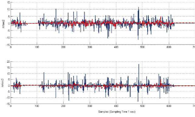
Fig.5. Bounds for dynamic error margins for accelerations along X (top) and Y (bottom) channels; along with real-valued observations are plotted in red.

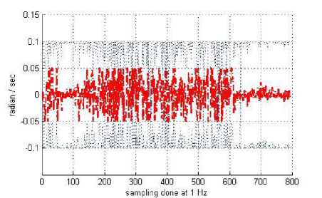
Fig.6. Bounds for dynamic error margins for angular rate about z axis (rate of change of heading of the vehicle); along with real-valued observations are plotted in red .

On the other side bounds of non-stationary error for rate gyroscope are found to be in consistence with the intervals as predicted using stationary noise coefficients. The guaranteed intervals estimated by the proposed forward backward contractor, are close to 95% confidence levels of stationary errors computed over the sampling period. Moreover the mean interval estimated using proposed method is sharper than the 95% confidence interval based upon stationary error statistics. In the present context, it may therefore be observed that, the stationary error characteristics do not completely define the stochastic behavior of the sensor when put in non-stationary operation. It is therefore an effective means as to employ interval techniques in studying the stochastic nature of dynamic errors associated with low cost MEMs inertial navigation sensor.

• V.    Conclusion

An associated contribution is laid in connection to characterization of MEMs inertial motion unit using interval methods. Analysis of stationary errors and determination of static accuracy is prominent in the literature. However, dynamic accuracies tend to vary due to angular variations incurred during motion of the platform. The present work involves forward and backward contraction of error intervals. An INS / GPS framework is considered for the purpose. Measurements coming from both the sensors are converted into intervals and fed into transition equations for extrapolation of state variables. The predicted intervals are contracted using GPS based position intervals. Subsequently, the contracted intervals are propagated backwards through first and second order derivations, and intersected with primitive inertial measurements obtained from the INS. The difference is obtained as an error interval for linear accelerations and angular rate. It is found that the proposed interval approach is instrumental in estimated dynamic errors of accelerations, such that they are inclusive of 95% confidence interval of stationary errors. This indicates a significant drift of dynamic error in accelerations which may not be clearly defined using stationary error bounds. On the other side sharper intervals are obtained for mean gyroscope errors in comparison to the predicted stationary bounds

Acknowledgment