Stochastic simulation of covariance matrix and power load curves in electric distribution networks

The adoption of automated meter reading (AMR) systems in the industry makes it possible to store statistical data about power transmission and consumption. Based on the above-mentioned systems and modern mathematical methods, it is possible to solve a series of problems: multifactor simulation, prediction and standardization of energy consumption and some integral characteristics of power systems; production activity analysis and optimization of power system functioning; diagnostics of electrical equipment in electric power supply systems etc. [1–3].

Power supply continuity and safety of electric power supply depend on a stability of a whole chain: “electric power generation – transmission – distribution”. Electric distribution networks, which are the master link in that chain, are the most problematic ones and outlay elements influence not only the electricity tariffs, but also the economic efficiency. About half of the current power sector’s basic assets are related to electric distribution networks, and most of the energy is lost just in these networks. However, the role of the electric distribution networks is still often underestimated on the background of global construction problems. Thus, dangerous and far reaching consequences, both economic and social, may arise [4].

Recently, taking into account the new computer technologies and the development of modern control measuring systems, the models of power consumption have been mainly developed by means of stochastic methods of component analysis, which include the principal component method [1, 5–12]. The models of power consumption or, in other words, the models of power load curves are able to decrease the volume of initial information needed for problem solving, and to simplify analysis of multivariate operating conditions in electric distribution systems. The problems include determination of power integral characteristics (energy losses, ranges of changing the operating condition parameters in the electric nodes and between power systems etc.), and reactive power compensation, both of which are very important when it comes to the complex optimization of power system and energy saving.

Deterministic methods, statistical simulation of power operating conditions, and determination of integral characteristics in power engineering have been advocated by different authors for some years [1, 5–8, 10–12]. The related research studies faced some difficulties: large dimension of the nodal power covariance matrix, large volume of information about power loads and operating condition parameters, complicated processing of initial information as well as underdevelopment of measuring systems, computers and programming. Therefore, the application area of stochastic analysis methods was limited. More recently, taking into account the adoption of SCADA and AMR systems, the above-mentioned disadvantages have been gradually disappearing, and the development of stochastic methods, partially the methods based on the principles of factor analysis, is more promising [13].

Conceptual Description of Principal Component Method

A component analysis as a method was developed by Pearson1; he proposed a method of databank compression which allocates a maximal variance. This method was also developed by Hotelling2.

The factor analysis is a multivariate analysis which researches an internal structure of the covariance or correlation matrices. It is applied for the statistical research of a system of random variables which have a correlation by means of stable random or nonrandom factors [9].

The principal component method is based on simple and ordinary conceptions, which depend on the covariance matrix analysis and the matrix linear transformation.

The modeling, characterizing the behavior of a random variable, is implemented by different ways of regression and factor analysis. In regression analysis the factors and model structure are entered a priori; in factor analysis we assume that, factors exist while their exact number and the model structure are only determined during the process of problem solving.

The principal component method is a dismemberment of a covariance matrix on the orthogonal vectors (components) or directions corresponding to the number of variables. These vectors correspond to the eigenvalues and the eigenvectors of the matrix. We agree that by a characteristic value we mean the set of eigenvalues and eigenvectors of the matrix.

Based on this method, the characteristic values are formed in descending order, which is important since only few components have to be used for the description of the initial data. The vectors are pairwise orthogonal ones, and their components are uncorrelated. A few components can reflect most of the sum variance of initial variables; however, all components are required for accurate reproduction of correlations between variables.

The principal component method is used for total simulation of initial random variables. However, we do not need to put forward the hypotheses about variables because the variables do not even have to be random variables. In practice the observations of random variables are samples from some population.

In order to decrease the complexity of the statistical calculations we can replace an n -dimensional random variable by k < n linear functions from the initial variables. The simulation is called a reconstruction of function using a linear predictor³, which is implemented by means of eigenvectors of the covariance matrix [12].

Consider the multivariate random variable X which is an n-dimension sample data x11

^x 12

x 21 ^... x n 1

x22 ... xn2

x 1 m x 2 m ^... x nm

For the analysis of other random variables depending on X , it is necessary to determine the mathematical expectations, for instance, sample mean or average values МХ 1 , МХ 2 , …, МХ n , and variations (changing) of initial random variables in the neighborhood of their average values Δ Х ₁, Δ Х ₂, …, Δ Х n . A characteristic of a random variable variation in the neighborhood of their average values is a variance . It may be that the linear combination of initial random variables has the maximal variance (certainly, we should compare only the normalized linear combination of random variables because any random variable can be multiplied by a large number, so any large variance can be obtained).

The linear transformation of initial variables is implemented by means of uncorrelated and normalized linear variables υ .

Linear Combination of Random Variables with Maximal Variance

Consider the possible linear combinations of random variables X _i

where X1 - x11 x12 x1i • X = k ■ Xk 11 xk 2 xki •U1 [""" U12 "1, • uk- Uk 2" .., . x. J _ Xk. J ... U1 m J ... _Ukm _ taking into account a limitation which fulfills the following condition of normalization m2

^ ^и = 1,       = 1,2,...,

1 =1

The variance of the linear combination (1) is determined by the following formula based on [7,

12]	о 2 G = DG =	^ 11 U 21 ...	U 12 -"- U 22 ... ...       ..	° 1 m U 2 m ....	x K(X) x	U 11    U 21  - U 12    U 22   . ...       ...	. " 1 . U k 2 ......	—
		U 1	U k 2   ...	U km J		U m   "  2 m	- Ukm J
								(3)
					" A 0.0	... 0.0 "
					0.0 a	... 0.0
		T = и	x K(X)	x u =	2	,

_0.0 0.0 ... A _ where K(X)=K - covariance matrix of initial random variables X1, X2, _., Xk;

k - rank of matrix K(X) ;

т – index of the transpose of a matrix;

m – total number of changing of the random variable Х i .

We assume that the matrix’s elements k ( X _i X _j ) are the estimations calculated from samples: x _{i 1}, x i 2 , …, x im and x j 1 , x j 2 , …, x jm . Thus, the selection of a random factor having a maximal variance is found through a minimum of function (3) satisfying condition (2). The optimization problem is solved by a method of Lagrange multipliers. Introduce an auxiliary objective function, which is Lagrange function

Ф = σ ² G + l ₁ ∑ ( υ ₁ ² _j - 1),                                                        (4)

where l 1 – the Lagrange multiplier.

An absolute minimum of the function (4) corresponds to the conditional minimum of function (3) subject to condition (2). The function including all variables is differentiated; the minimum condition is obtained as

_∂ ^∂ _υ ^Ф = 2 ∑ ^mK jr υ 1 j - 2 l 1 υ 1 r = 0; r = 1,2,..., k ; ∑ ^m υ 1² j = 1.                             (5)

r         j =1                                                                     j =1

The solutions of system (5) are all normalized eigenvectors of the matrix K(X). Every solution determines an extreme point or specific point of the function. The coordinates of the eigenvector corresponding to the maximal eigenvalue λ₁ correspond to the global minimum.

In factor analysis the components of the vector G are new random variables which are the linear combination of initial X or centered АХ random variables.

The eigenvalues λ and eigenvectors υ of power covariance matrix have useful properties which are applied in component analysis. The eigenvalues are real values and the eigenvectors can be chosen as perpendicular to each other. The eigenvectors define an undergoing pure tension or compression direction of the linear transformation corresponding to the matrix K(X) . These vectors are also named the principal components of the matrix [12], and the eigenvalue λ is a coefficient of the transformation. The variance of the i -th principal component is equal to the eigenvalue λ_i of matrix K(X) .

It is known that the eigenvalues λ and eigenvectors υ of matrixes satisfy the following expression

К х и = и х X .                                                                (6)

By multiplying both sides of the expression (6) on the left of the matrix υ ^-1 , we will arrive at

X = и ^-1 X K X и .                                                                  (7)

Expression (7) is considerably simplified when the original matrix K is defined as positive, which is the case for the power covariance matrix [7]. Thus, all eigenvectors can be made orthonormal ones, i. e. satisfying the expressions

υ i ^т × υ j = 0 when i ≠ j ; υ i ^т × υ j = 1 when i = j .

It is easy to verify that the inverse matrix υ ^-1 is equal to the conjugate one, and expression (7) can be rewritten as (3)

X = ^{и т} х K х ^и ,                                                              (8)

where и - an orthonormal matrix whose columns consist of eigenvectors u 1 , и 2 ,..., u k . Condition (2) is satisfied for every column of the orthonormal matrix.

Inverse expression between the original matrix K and the matrix λ

	r K = [ U 1	U 2	... U k ]x X x U		2	... U k ]     ,
U 11 U 12	U 21 ... U k 1   " U 22 ... U k 2 22       k 2		Л 0.0.. o.o л . 2 2	.0.0 " .0.0		U 11   U 12 ... U 1 m " U 21 U 22 ... U 2 m	.                                      (9)
... U 1 m	... ...... U 2 m ... U km -1	x	...... . 0.0 0.0.	..... .. л	x	...... ...... L U k 1 U k 2 ... U km \

The method allows us to select the orthogonal factors among the factors-arguments, i. e. statistically-independent components, which provide a linearity of the method and additive efficiency.

The above-mentioned properties of the eigenvectors show that the full totality of them is equivalent to the original probabilistic model corresponding to the vector X. Moreover, both sets , of variables X and G define the same vector space.

However, from the set of vectors G , it is sufficient to select a small number of M principal components (factors) explaining most of the relationships between all components of the initial vector of random variables X . The main factors are not directly observed, but they characterize the change in the original variables. Therefore, we can get the task of obtaining a linear predictor of dimension M ( M < k ). For each k , the best predictor is the first M eigenvectors of K , corresponding to the maximal eigenvalues. As a result of studying the internal structure of the matrix K , the selection of main factors is made in such order that at the beginning the first of them makes the greatest contribution to the variance of the variables, then the second one is the largest contribution to the variance of the variables remaining after taking into account the main factor, etc. Ultimately, these vectors constitute a set of linearly independent basis vectors, oriented in such a way that each of them makes the maximum contribution to the variance of the original variables Х .

On the practical side, the factor model makes it possible to adequately estimate the covariance structure between the relatively large number of observed variables by means of a smaller number of common factors. Evaluation of the factor structure is carried by the required number of factors explaining the correlations between variables and load factors in these variables. Component analysis is most useful when all variables xi are measured in the same units. If not, the method is much more difficult to validate [9].

Factorial or component methods of statistical analysis are used in the computation of operational energy losses [13, 14], as well as for short-term forecasting and optimization [15, 16]. When solving the problem of factorial simulation of electric loads via a stochastic approach, the information about the characteristics of the random variable is approximately determined by a partial sample from the general population. In the factor simulation of power loads [5–7, 10, 11] the curves of active and reactive nodal powers are considered as a training sample having 2 n -dimension. In operational computations the scope of the method is limited to the modeling of daily power load curves of an unobservable network.

The modeling of electric power loads on the basis of factor analysis allows us to:

• –    find hidden regularities, which are determined by many internal and external causes of load changing;

• –    carry out the compression of information by describing all curves by means of the common factors or principal components, whose number is much smaller than the number of initial curves;

• –    identify the statistical dependence between the power load curves and the main factors;

• –    predict the random component curves based on the regression equation constructed on the basis of factor analysis;

• –    simplify the methods for determining the integral characteristics of power systems.

Determination Methods of Principal Components

The problem of determination of the principal components is a classical problem of determining the characteristic values from a covariance matrix of random variables, as which the nodal power loads are considered. The determination of eigenvalues and eigenvectors of matrices in linear algebra is called the problem of characteristic values , and it is a complicated task which is implemented in several statistical software applications. The value λ is called the eigenvalue of K , if there is a nonzero vector (eigenvector of K ) satisfying the equation

( K - Ax E ) X и = 0,                                                         (10)

where E – unity matrix; 0 – null vector.

The system (10) is a homogeneous system of liner equations because the free members of its equations are zeros. It has nontrivial solutions if the determinant of matrix |K - Ax E| equals zero, i. e.

A" + PA ^-1 + в ₂ A"-2 + ... + p „-1 A + p „ = 0,                                      (11)

where p 1 ,..., p n - coefficients of the characteristic polynomial.

The methods for determining the eigenvalues and eigenvectors can be divided into two groups [11]: the first group includes iterative methods which often use a similarity transformation and solve a linear system of equations (10); the second group includes the direct methods that calculate the characteristic polynomial (11). The problems (10) and (11) have different conditionality, as the roots of polynomials (11) are often highly sensitive to errors which are inevitably arising in the calculation of polynomial coefficients. That was the main reason of the almost complete exclusion of direct methods.

The direct application of covariance matrix in various algorithms is greatly complicated by its dimension. In order to compensate the above-mentioned disadvantage, the modeling of covariance matrix is implemented by using modern computer software interactive systems, such as MATLAB, MATCAD, C++, ANSYS, FORTRAN, etc.

The main criterion for the normalization of the eigenvectors in MATLAB consists of ит х и = E.

Small changes in matrix elements, such as rounding errors, can cause large changes in the characteristic values. The power covariance matrix is a square matrix that is easier to use for matrix transformations in comparison with other matrices.

Stochastic Model of Covariance Matrix and Electric Power Loads

Most of the research [5–8] conducted in this field was aimed at the modeling of power loads and its application for a daily time interval. This is due to the peculiarities of the energy business and information support of power utilities during the development of this technique. Structural changes that have occurred in the management of an integrated power grid led to the need of periodic computations between separate power business entities. Today, the main period of the financial settlement is one month. The modeling of power consumption on a monthly time interval was proposed for the first time in [10, 11]. At the moment the technique and its possible application are implemented insufficiently and therefore further research and elaboration is needed.

The simulation of the power covariance matrix is based on several properties of eigenvalues and eigenvectors of a matrix which is expanded by 2 n eigenvalues and eigenvectors; the first few M characteristic values ( M <<2 n ) accurately reflect the total variance of the initial power load curves [5–7, 10–12].

Statistical analysis of power operating conditions uses information about variances of power loads с2Pi, ст2Qi and cross-covariance functions k(PiPj), k(PQj), k(QQj) between random variables of different power nodes dd

^ ² P i = 7 £ ( P im — MP i ) ; ^ ² Q i = £ ( Q im - MQ.) , i = 1, n ;

d m = i                              d m = i

d tlP^ - d SP - M e, - m^.m- i.-;

m - 1

d

k ( PP ) - 7 £ ( P im - MP i )( P jm - MP j ), i , j - 1, n , i * j ;

d m - 1

m - 1

1 ^d

k I Q i Qj^ Z-Q m ⁽ Q- ^- Me , )! e, ^- MQ j ), I,) ^{- 1},n , i * j. d m - 1

m = 1

where i , j – indexes of nodes; m – index of every time interval for the T period; n – the number of nodes of power distribution systems with known or simulated power load curves.

The elements (13) of a power covariance matrix characterize the degree of irregularity of power load curves, which remains approximately constant over a long period. The degree may be determined on the basis of daily measurements performed on different days in power system sectors. This is an important advantage of the statistical method.

The variances and cross-covariance functions of power loads form the square covariance matrix K = K(P,Q) as follows

K(P,Q ) =

K 11

K ₂₁

K ₁₂

K ₂₂

0 2 P k ( PP 2 )...... k ( PP )		Г k ( PQ i ) k ( PQ 2 )...... k ( P i Q n ) 1
k ( P 2 P 1 )   0 P2......k ( P 2 P n ) 21       2        2 n		k ( P 2 Q i ) k ( P 2 Q 2 )...... k ( P 2 Q n ) .................................................
.......................................... k (^ k ( P n P 2 )...... ° 2 P n ^		L k ( P n Q i ) k ( P n Q 2 )...... k ( P n Q n ) J
k ( Q 1 P 1 ) k ( Q 1 P 2 )...... k ( Q 1 P n )		1	‘0 2 Q i k ( Q i Q 2 )...... k ( Q i Q n )
k ( Q 2 P ) k ( Q 2 P 2 )...... k ( Q 2 P n ) ..........................................			k ( Q 2 Q i ) 0 2 Q 2 k ( Q 2 Q n )
k ( Q n P ) k ( Q n P ^ )......k ( Q n P n ) J			k ( Q n Q i ) k ( Q n Q 2 )...... 0 2 Q n

The simulation of the covariance matrix is implemented corresponding with expression (9), which may also be written in the usual form

M

K = У A x и x U . iii i=1

Every eigenvalue of covariance matrix corresponds to a general load diagram of power (GLD) Г_i , which is a linear combination of 2 n initial nodal power load curves centered at expectation MP i , MQ i

where [ u_2n ] ^т - the transposed matrix of eigenvectors obtained from the covariance matrix of statistical sample for initial power loads, which has 2 n ×2 n dimension;

Δ Р ₁ , Δ Q ₁ – the deviations centered at expectation of active and reactive power in the node # 1 for

a certain time period T				, m =1,2’'	, d
N P 1 =	"A p 11 " A P 12 A p 13	, A Q1 =	" A : 12 A q 13
	.... _A P 1 m _		.... A q 1 m

The obtained GLDs can be considered as new independent centered random variables with zero mathematical expectations. The GLDs have a property of orthogonality, i. e. cross-covariance functions k ( Г i Г j ), k ( Г j Г i ) are equal to zero. These new random variables (factors) are a suitable coordinate system for accurate simulation of initial random variables P i , Q i ; therefore, using M of them

Г_k = [ Г 1 .... Г k ] << Г_2n , k = 1,..., M <<  2 n ,                                         (17)

which corresponds to the maximal eigenvalues of power covariance matrix, allow us to simulate initial load changing with a sufficient accuracy for a certain time interval T

• = ONE_m ,1 x [ MP_V...MP n MQ_V..MQ n ] + Г x [ u k ] т = [ P ... P n Q_V.Q ] , k = 1,..., n ,

where ONE _{m ,1} – a column vector consisting of units, and which have m = 1, 2,..., d rows.

[ u k ] ^т - the transposed matrix of prime k eigenvectors U k corresponding to the first maximal eigenvalues X _t of the power covariance matrix K(P,Q) ⁽1⁴⁾;

MQ 1 – a mathematical expectation of reactive power curve in the node #1 for the accounting period T .

Р i – possible variation of active power in i node for the accounting period T .

The simulation of the power loads allows us to track the variation of load parameters. It should be noted that initial power load curves are fully simulated on formula (18) using all GLDs. The eigenvalues X of the initial covariance matrix K(P,Q) are variances of GLDs (3). Hence, any power load curve can be represented as a linear combination of the GLDs which reflect the general regularities of power expectation changing for the initial collection of power nodes.

The following daily/monthly samples of the power load curves have been analyzed:

• 1)    36 simple weekday and weekend power curves [24 hrs] of a 10 kV electric distribution network ( d =4); the unit of active power is kW; the unit of reactive power is kvar.

• 2)    18 atypical real daily active and reactive power curves of a 10 kV electric distribution network ( d =24) [11]; the unit of active power is kW; the unit of reactive power is kvar.

• 3)    42 typical daily power curves for different industries ( d =12) [12]; the unit of power is relative unit [r. u.].

• 4)    30 monthly active power load curves for 110–220 kV overhead lines for August–September in 2009 [11]. Number of intervals d of period T was reduced from 744 to 31 by calculating the average power for each day. The unit of active power is MW.

Computational results of eigenvalues and GLDs (17) from the above-mentioned samples of data #1–4 are presented in Table 1–3, and in Fig. 1–2.

The original power load curves characterize a different degree of irregularity, therefore every sample data #1–4 has its own principal factors linking the power load curves to the system of characteristic values. In all cases, the error of simulation of power load curves is, in a dozen times and sometimes more, less than the error of the covariance matrix simulation (9) taking into account

Table 1. The Six Maximal Eigenvalues Obtained from Sample Data #1–4 for Simulation of Covariance Matrix and Power Load Curves

Sample Data	Contribution of principal components to the total variance of loads	Eigenvalues of the original sample data in decreasing sequence
		λ 1	λ 2	λ 3	λ 4	λ 5	λ 6
1)	λ	45806.73	25494.41	5039.49	4.64∙10-12	-	-
	Θ , %	60.00	33.40	6.60	0.0	-	-
2)	λ	17699.71	9289.16	2247.51	1136.81	595.20	502.52
	Θ , %	53.28	27.96	6.77	3.42	1.79	1.51
3)	λ	1.06705	0.432602	0.104090	0.102429	0.0284292	0.0157218
	Θ , %	60.10	24.36	5.86	5.77	1.60	0.885
4)	λ	1510.38	369.29	172.26	80.00	68.83	47.70
	Θ , %	65.06	15.91	7.42	3.45	2.96	2.05

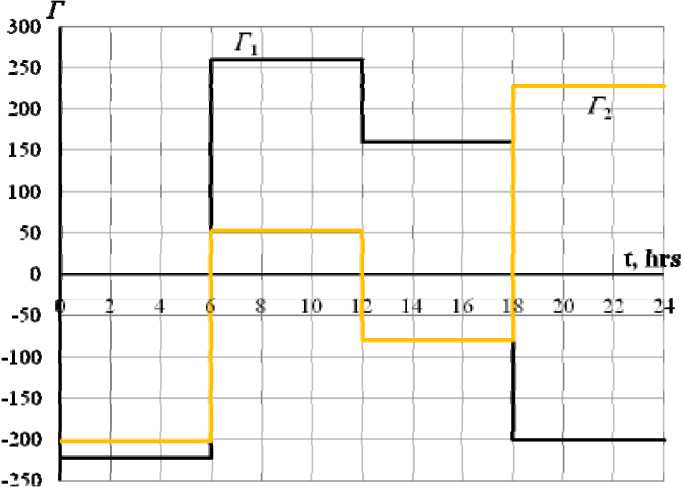
Fig. 1. Two Principal Daily GLDs Corresponding to the Maximal Variances for Sample Data #1 in the Same Units as the Initial Variables

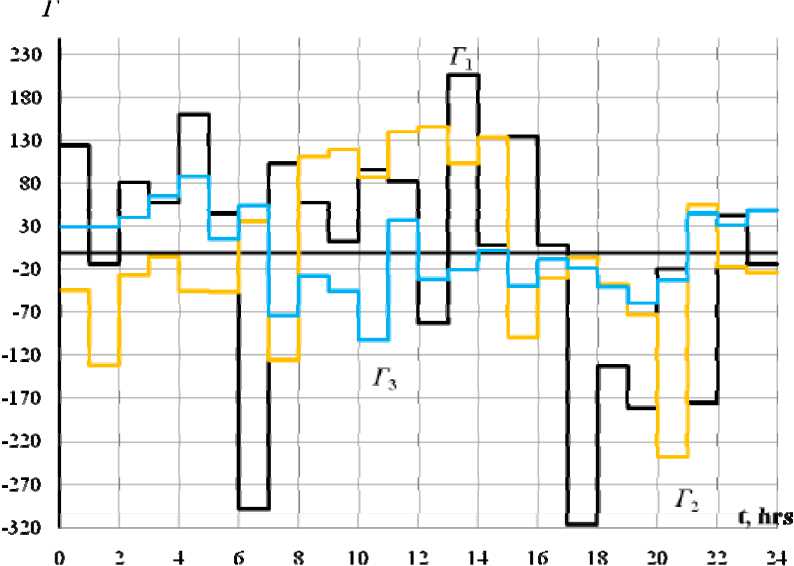
Fig. 2. Three Principal Daily GLDs Corresponding to the Maximal Variances Obtained from Sample Data #2 in the Same Units as the Initial Variables

Table 2. Six Daily Nonnormalized GLDs Corresponding to the Maximal Variances Obtained from Typical Daily

Power Curves for Different Industries (Sample Data #3) [r. u.]

t, hrs Г1 Г2 Г3 Г4 Г5 Г6 0–2 -1.58281 0.107604 -0.184982 0.0774817 -0.00315256 0.0536194 2–4 -1.63002 0.111508 -0.193562 0.0402251 0.0274119 0.0268668 4–6 -1.00645 -0.0537509 0.339956 -0.721240 0.201227 -0.130268 6–8 0.826063 0.369511 -0.435288 -0.464289 -0.383642 0.0144767 8–10 0.965881 0.888987 0.169168 0.111077 -0.0132479 -0.241056 10–12 0.186023 0.684827 0.589090 -0.0899582 -0.0842728 0.267227 12–14 0.671946 0.990801 0.0328418 0.464211 0.1607393 0.00610122 14–16 1.33107 -0.155875 -0.588556 -0.189836 0.303330 0.0769681 16–18 0.832963 -1.12614 0.168255 0.0598246 0.0587576 0.125265 18–20 0.687673 -0.991643 0.289502 0.0722762 -0.101288 -0.107512 20–22 -0.0217858 -0.704435 0.00610245 0.325773 -0.0908384 -0.0676617 22–24 -1.26054 -0.121393 -0.192526 0.314455 -0.0750239 -0.0240258 the same number of characteristic values and GLDs. The reason for this is that the elements of the power covariance matrix are relatively small values compared with the values of the initial power load curves. The maximal error of simulation of power load curves does not exceed 25%, and the average one is 8.83% for sample data #3 taking into account only six maximal characteristic values.

The obtained GLDs can also be used to determine the total normalized or weight average GLDs which are used for the simulation of unknown power load curves.

By the means of MATLAB system using all GLDs and characteristic values for the sample data, the power covariance matrix (9) and power load curves (18) are simulated with high accuracy. The simulation on the basis of expression (18) is primarily designed for modern automated meter systems and it uses operating condition information from them. The lack of the above-mentioned systems in most distribution systems can be replaced by the power load simulation [7, 11] and so to use the advantages of factor simulation.

Stability of Factor Power Load Model

Factor simulation of power loads has a practical application only if the estimations of factor values (GLDs), which are obtained for different random processes of load changing, are statistically similar ones, i. e. have statistical stability. A research study of the statistical stability of the factor model, which was based on real data on power load curves for different power utilities with large statistical volume of information, showed the presence of a collective and dynamic stability for daily, weekly and monthly power load curves [4, 5, 7, 10, 11].

Statistical stability describes the possibility of using GLDs derived from one learning sample for the simulation of powers which were not included in the learning sample. Dynamic stability describes the comparison of different time realizations of the factor model for constant power utilities; collective stability is the comparison of GLDs belonging to different power utilities.

Table 3. Six Monthly GLDs Corresponding to the Maximal Variances Obtained from Sample Data #4 [MW]

d	Г 1	Г 2	Г 3	Г 4	Г 5	Г 6
1	-61.0910	-19.4337	-5.91616	0.987755	-17.5551	2.85404
2	-49.9621	-17.3637	0.624555	6.63003	-10.2079	-7.32189
3	-56.1344	-11.5625	10.9850	9.11488	-9.88028	-11.2969
4	-44.3974	-8.20962	10.8664	5.96288	0.0544416	-17.9550
5	-29.6979	2.44294	-19.8471	8.92353	-2.01733	2.65349
6	7.69728	16.7571	-23.6115	8.33256	-4.15039	9.31310
7	50.0524	42.8409	0.189204	4.71245	-14.7875	-3.14985
8	51.1595	42.7496	-11.1642	-6.21158	-10.4222	-7.43516
9	54.5808	14.4466	-22.6867	-2.33433	6.02504	-11.5762
10	43.7955	-33.5056	-13.8767	4.15772	2.12694	-4.75286
11	42.7563	-28.2635	-14.5850	4.16292	2.03908	-4.62368
12	22.2479	0.475527	-4.00582	-13.7653	-16.9796	3.54289
13	-82.9028	22.9289	8.61478	-27.3533	-3.32166	-0.580486
14	-89.8760	32.9555	-14.5703	2.33812	20.4750	4.03684
15	-64.0213	8.74729	-18.2781	11.1739	4.56532	4.64756
16	24.1308	-4.13785	-10.5377	8.70718	8.82819	0.635262
17	7.18290	-15.8651	8.20768	-3.85646	7.90065	-5.18798
18	6.47624	-14.2352	3.61354	-9.05050	8.53147	-5.94042
19	11.5967	-4.96041	-1.97678	-11.5722	5.81598	-2.55565
20	13.6620	-8.57086	-3.04740	-12.5938	5.49477	-0.341653
21	9.67771	-13.5638	-3.17290	-11.0283	3.86244	2.55857
22	8.28646	-17.2128	1.59427	-6.97636	3.11115	2.62101
23	3.85626	1.39991	11.8803	0.615213	-1.67941	3.97740
24	11.9982	-10.1443	8.96102	4.82252	-3.59272	6.98522
25	14.4479	-15.7646	12.6704	5.13767	-0.285371	7.41964
26	14.5485	4.14165	10.7802	-1.09407	2.70395	8.33036
27	19.7817	15.1572	24.4290	9.36452	4.34313	-0.319466
28	19.8501	26.3028	27.7652	14.1172	2.67827	-0.136420
29	17.8695	5.40787	15.9846	1.12875	7.99281	1.50315
30	15.8722	5.87849	9.71566	-4.84532	5.26982	5.52796
31	6.55574	-19.8384	0.394553	0.291731	-6.93900	16.5671

The research studies of daily power load curves obtained by the AMR system in more than 100 points of head line sections in 6–110 kV distribution networks for 13 days identified a strong statistical relationship between the first GLDs, i. e. proximity of variances of the power load curves and close correlation dependence [11]. This allows us to conclude that the factor model of the covariance matrix and power load curves have statistical stability, and it is possible to apply it for the simulation of power consumption irregularity for the posterior or previous analogous time periods.

The results of multiple computations indicate a rather large contribution of the three principal components (70–80%) to the total variance of the whole sample of original power load curves. The first – 50 – principal components of GLDs indicate the presence of common internal reasons for daily irregularity in power load curves and intersystem power flows [6].

The collective stability of the factor model allows us to suggest that GLDs reflect the main reasons for power changing without specific factors. Therefore, in order to determine the GLDs, we do not need to analyze the power load curves in all nodes; it is enough to take only some modeling subset of power load curves into account, for instance, combined diagrams of consumer groups. These are formed on the basis of check measurements of power consumption, which is carried out by an inspectorate. The computation results showed that sets of GLDs which were obtained on the basis of analysis of large samples of power load curves are quite close to each other [6].

Computations for different samples of daily and monthly power load curves have also confirmed the statistical stability of the factor model (see above). The contribution of the first principal component to the total variance of power loads is over 50%, while the significant contribution of the first three components was also confirmed (see Table 1).

Wide application of factor analysis for power load simulation offers a possibility to limit the volume of the statistical sample to not more than 100 elements [7, 8], which allows to manipulate not large covariance matrices. In this case, the requirements of representativeness are carried out, and the obtained GLDs are statistically stable diagrams.

A Number of Principal Components

A recent review of the approaches to determine the required number M of eigenvalues and eigenvectors for covariance matrix simulation identified the absence of a consensus among specialists on the factor analysis [11]. One opinion is that this number is usually not higher than four. However, in some cases depending on the accuracy of the covariance matrix simulation, it is required to take into account a greater number of characteristic values and GLDs. Researches of power covariance matrix and power load curves showed that the required number of characteristic values depends on sample data properties and on the irregularity of power load curves. The maximal number is equal to the first six maximal characteristic values in MATLAB system. Most likely, this number was chosen after extensive analysis of covariance matrices and factor simulation.

A simple approach for the determination of a reasonable number of characteristic values is to estimate the overall contribution of the principal components’ sequence Г ₁ , Г ₂ ,..., Г_k to the total variance. If the summarized contribution to the total variance is 75–90%, we should stop on the value k =1, 2,…, М [5, 6]. The total percentage contribution Θ to the variance for fixed M is calculated by the following formula

M

∑ λk

Θ = ^{k =1}    ⋅ 100%; 75 ≤ Θ ≤ 90%,                                           (19)

2 n _λ

• ₂                   ^∑ i =1 ^{λ i}

where ∑ λ _i – the sum of eigenvalues of original power covariance matrix, which is called spur of i =1

matrix [7, 8]. Θ is a criterion for the accuracy of the covariance matrix simulation and the simulation of original active and reactive power load curves. This criterion is sufficient to carry out the computations of the power integral characteristics and power system optimization.

Component analysis is used to simulate both random and deterministic dependencies similar to the regression method of approximating the functions dependent on the time. The most effective test of statistical hypothesis and the determination of the required number of principal components is the repeated application of component analysis for various samples of the same general population. If the statistical hypothesis about the existence of common dominant trends in all random variables Х _i is true, then the statistical characteristics, at least for the first principal component selected on the basis of different sample data, will be close to each other.

The statistical characteristics for principal components Г k not characterized by the properties of one general population differ substantially from sample to sample. Repeated factor simulation for different sample data is a universal method to select statistically stable principal components which characterize the properties of the general population.

The factor simulation of a set of random variables is a useful instrument of statistical analysis if the dimension of the model space of M initial random variables is a sufficiently small one. Such a situation is typical for the simulation of nodal power loads. The application of factor analysis methods allows us to simulate hundreds of power load curves by the means of 2–3 GLDs [7, 8].

For a reliable application of the method, it is necessary that the first eigenvalues of the K are significantly different from each other. The matrix K , which corresponds to the nodal power load curves, usually satisfies this condition [12].

The required number of GLDs for the simulation of original power load curves or required number of characteristic values for the simulation of power covariance matrix depends on the properties of the concrete set of research random variables. The research studies on different collections of power load curves confirmed the hypothesis about high quality simulation of power covariance matrix. This simulation is based on a small number of characteristic values reflecting the maximal part of the total variance for the whole general population; hereby a small number means 2÷5 GLDs, the exact number depending on the properties of the sample data, desired accuracy and purposes of simulation.

Stochastic Simulation of Covariance Matrix and Power Load Curves’ Algorithm

Referring to the above-mentioned points we can formulate a simulation algorithm for covariance matrix and power load curves:

• 1.    The original power covariance matrix K(P,Q) is formulated on formulas (13), (14) based on retrospective analysis of active and reactive power curves in distribution networks for a certain time period T and control measuring data.

• 2.    2 n eigenvalues and 2 n eigenvectors of the K(P,Q) are determined by means of any suitable software based on the principal component method. The characteristic values identify a degree of statistical relationship between random deviations of powers P i , P j , Q i , Q j from their mathematical expectations MP _i , MP _j , MQ _i , MQ _j .

• 3.    A selection of first M maximal eigenvalues of the K(P,Q) λ k < λ and eigenvectors υ k <  υ is arranged in descending order. The number of eigenvalues and GLDs needed for covariance matrix simulation is an acceptable one for practical computations of integral characteristics and system optimization if condition (19) is satisfied. In other words, we should stop on such value of M where the contribution of sum of the first diagonal elements of the covariance matrix to the total variance – 52 –

• 4.    The simulation of the power covariance matrix K(P,Q) is carried out on formula (9) by the means of M characteristic values. Computations like that can be performed only once a month based on the analysis of a training sample of power load curves.

• 5.    The GLDs are determined on formula (16) for the whole collection of the corresponding sample data.

• 6.    The first M maximal GLDs Г k are selected on (17), which correspond to the M eigenvectors υ_k and eigenvalues λ_k of K(P,Q) . The original active and reactive power curves are simulated on the expression (18) by the means of Г k .

of the general population of active and reactive powers is 75–90%. The recommended range of M is 2 ≤ M ≤ 5.

This method is effective when the condition М <<2 n can be limited to take into account only the first few υ k and Г k . In addition, the GLDs Г k obtained for the different random process realizations of power load changing must have statistical stability. The property of universality was confirmed by means of computations of the GLDs Г k of statistically representative sample data for different power utilities. In all cases, 3–4 Г _k are usually sufficient for the reflection of up to 75–95 % of the total variance of original power loads (see tab. 1–3).

Thus, the original power load curves can be presented in the form of some characteristics: the mathematical expectations and the coefficients λ k and υ k . This is used for effective determination of integral characteristics and optimization algorithm in power distribution systems.

In order to obtain a more accurate model of covariance matrix and power load curves it is necessary to take into account a larger number of characteristic values and GLDs, and it is possible to use the expansion in a Fourier series or similar methods [8]. However, the component analysis differs from other statistical methods by offering a more economical and convenient way for system optimization and a good form for the presentation of information. One advantage of the component analysis is that it is determined in such way that the function package of simulation is not selected randomly, as for instance, in Fourier analysis, but on the basis of analyzing the principal regularity of power load changing. The indicated regularities obtained on the basis of the main factors, their number is less than in other simulation methods, determine the possibility of their application for small samples containing 4–6 points of a daily curve.

The methodology of the integral characteristic determination is developed on the basis of stochastic simulation of covariance matrix and power load curves particularly the load-dependent energy loss determination [13, 14] and optimization algorithms of operating conditions on reactive power in electric distribution networks [15, 16].

Conclusions

• 1.    This paper proposes the factor model of power loads on daily and monthly time periods, which allows us to identify the general regularity of nodal power changing in electric distribution networks. The advantages and possibilities of the model application are described.

• 2.    The computational results of the general load diagrams are derived for different sample data of original active and reactive power curves for daily and monthly time periods T . The statistical stability of factor power load model is confirmed for 6–110 kV electric power networks. The contribution of the first principal component to the total variance of power loads is more than 50%.

• 3.    The simulation algorithm for covariance matrix and nodal power load curves is formulated by means of only a subset of the first main factors (2 ≤ М ≤ 5); it is possible to decrease the complexity of computations in comparison to traditional computation of multiple operating conditions and to simplify the determination of power integral characteristics.

• 4.    The algorithms of energy loss determination and ranging of reactive power changing are developed on the basis of the proposed stochastic model of covariance matrix and power load curves [13–16]. This can be effectively used for solving the problems of energy saving and power system optimization.

A.V. Tihonovich, Calculation of Energy Losses Based on Deterministic and Stochastic Methods and Algorithms in Electric Distribution Systems/ PhD Thesis Summary. Krasnoyarsk, 2008, 20 p.

• [12]    Герасименко А.А. Применение ЭЦВМ в электроэнергетических расчетах: учеб. пособие. – Красноярск: Изд. КПИ, 1983. – 116 с.

A.A. Gerasimenko, EDC Application in Power Engineering Computations// Tutorial Book, Krasnoyarsk, 1983, 116 p.

• [13]    Герасименко А.А., Нешатаев В.Б., Шульгин И.В. Расчёт потерь электроэнергии в распределительных электрических сетях на основе вероятностно-статистического моделирования нагрузок: Известия высших учебных заведений. Электромеханика, 2011, № 1, С. 71–77.

A.A. Gerasimenko, V.B. Neshataev, I.V. Shulgin, Energy Loss Evaluation Based on Power Load Simulation in Electric Distribution Networks/ Proceedings of the Higher Education Institutions “Electromechanics”, 2011, #1, pp. 71–77.

• [14]    Герасименко А.А., Нешатаев В.Б., Шульгин И.В. Вероятностно-статистическое определение потерь электроэнергии в задаче оптимальной компенсации реактивной мощности в распределительных сетях // Энергетика в современном мире: материалы IV Всероссийской научно-практической конф. Ч. 1. Чита: ЧитГУ, 2009. С. 214–221.

A.A. Gerasimenko, V.B. Neshataev, I.V. Shulgin, Stochastic Determination of Energy Losses in Optimal Reactive Power Compensation Problem in Distribution Networks/ Power Engineering in the Modern World/ Proceedings of IV All-Russian Scientific Practical Conference. Vol. 1. Chita: Chita State University, 2009, pp. 214–221.

• [15]    Герасименко А.А., Липес А.В. Оптимизация режимов электрических систем на основе метода приведенного градиента // Электричество, 1989, № 9. С. 1–7.

A.A. Gerasimenko, A.V. Lipes, Optimization of Power Operating Conditions Based on Reduced Gradient Method// “Electricity” Journal, 1989, # 9, pp. 1–7.

• [16]    Герасименко А.А., Нешатаев В.Б., Шульгин И.В. Оптимальная компенсация реактивных нагрузок в системах распределения электрической энергии// Известия высших учебных заведений. Проблемы энергетики. 2008. №11–12/1. С. 81–88.

A.A. Gerasimenko, V.B. Neshataev, I.V. Shulgin, Optimal Compensation of Reactive Power Loads in Energy Distribution Systems// Proceedings of the Higher Education Institutions. “Power Engineering Problems” Journal # 11-12/1, 2008, pp. 81–88.

Стохастическое моделирование матрицы корреляционных моментов и графиков нагрузок мощностей узлов распределительных электрических сетей

И.В. Шульгина,

А.А. Герасименко^а, Су-Чуан Джоу^{б a} Сибирский федеральный университет Россия 660041, Красноярск, пр. Свободный,79 ^б Харбинский политехнический университет КНР, Харбин