Structure design toolkit of quantum algorithms. Pt 1

The Hadamard gate creates the superpositions of classical states, and CNOT gate create the entangled states for robustness quantum computation. We consider the possibility of creation the interference with Quantum Discrete Fast Fourier Transformation (QFFT). Well-known examples of such transforms include the discrete Fourier transform (DFT), the Walsh-Hadamard transform, the trigonometric transforms such as the Sine and Cosine transform, the Hartley transform, and the Slant transform. All these different transforms find applications in signal and image processing, because the great variety of signal class, occurring in practice, cannot be handled by a single transform.

Quantum Parallelism, Interference, and QFFT.

We now have sufficient ingredients to understand how a quantum computation can perform logical operations and compute just like an ordinary computer [1-18]. We describe an algorithm, which makes use of quantum parallelism that we have hinted already: finding the period of long sequences.

Quantum Parallelism for Computation of Classical Functions. We use the fact that the efficiently implementable classical functions can be implemented with comparable complexity on a quantum computer using standard blocks. We assume perfect operations, so we do not deal with error control.

Remark. Let

f ( x )

be a classical polynomially computable function. Quantum parallelism can be used to compute all the values of f (x) for all x at the same time. We will ignore any temporal work space, which returns to its original state by the end of the computation that might be needed to compute f (x) . Knowing that arbitrary classical function f (x) can be implemented on quantum computer, we assume the existence of a quantum array U that implements f . What happens if U is applied to input in a superposition? The answer is easy but powerful; since U is a linear transformation, it is applied to all basis vectors in the superposition simultaneously and will generate a superposition of the results. In this way, it is possible to compute f (x) for all n values of x in a single application of Uy . This effect is called quantum parallelism and was in detail in Part 1 described.

We use the following standard transformation to implement the quantum parallel computation of f ( x ) , Uy :| x , yj ———> | x, y Ф f ( x ) where Ф does not denote the direct sum vectors, but rather the bitwise exclusive - OR. Operator Uy defined in this way is unitary for any function f ( x ) . To compute f ( x ) we apply Uy to | x ,0^ . Since f ( x ) ф f ( x ) = 0 , we have UyUу = I .

Graphically the transformation U is depicted as

I x) —— I y)—

U f

—    I ^х)

— |y ® f (x ))

Consider a superposition of x values, E ax | x^. Then Uy transforms Eax\x) ®| °)  as xx

E a x l x ’°)   > E a x I ^х ’ f ( ^x )).

xx

Example: Changing of sign. We still have to explain how to invert the amplitude of desired result using operator Uy . Let f (x) = 1 if the sign of x is to change, and f (x) = 1 otherwise. We show, more generally, a simple and surprising way to invert the amplitude of exactly those states with f (x) = 1 for a general f . Let Uy be the gate array that performs the computation Uy : | x, b ^ | x, b ® f (x)^. The additional register is set to the superposition b = -^=(| °) - Ц)• The operation Uy then gives a superposition in which the phase of those x with f (x) = 1 are inverted and |b) remains unchanged. This means that applying of Uy to the superposition E a* | x) and choose | b) as above to end up in a state where the sign of all x with x f (x) = 1 has been change, and b remains unchanged. This is readily seen as follows:

^U f [ E " x| x > ® ^ (I 0 - 1 ) ]

E a x l x ’°) ^- E a x l x ’0 + E a x l x ’0 ^- E a x l x ’°)

V x G X °               x G X °              x G X 1              x G X 1

[_.._. .Д 1

= E a x l x ) ^- E a x l x ) ®77⁽l °) -1¹))

V x G X°          x G X1       J V- where Xo = {x|f (x) = °} and X] = {x|f (x) = 1}. The operation introduces a phase factor of - 1 for exactly those x g X,, as desired. It also leaves | b^ unchanged. In particular the extra register is not entangled with the x values.

Remark. This technique requires only one call to U , but restrict the phase to 1 and – 1.

Example: Suppose we want to change the phase of all elements of X_v by у . Instead of using

;= ( ° -Ц) we use I b = —j= ( °^ + y| 1). The result of applying Uy is

^U f ^[E a x l x ) ® 4т⁽°)+ A ¹ ) V x           2 2           J

E a x I x ’°)+ y E a x I x д) + E a x I x д) + y E a x I x ’°) V x G X °                x G X °             x G X 1               x G X 1           J

In general, the resulting state is not simply a tensor product of x and b with some additional phase shift. Usually, x and b become entangled . A possible approach to extracting the desired state from entanglement is to measure the last bit. The state in last equation becomes either

[_.)

E a x l x ’°) ⁺ y E a x l x ’°)

V xG Xq              x G XxJ

or

[ y E axlx ’1+ E axlx ’1

V  x G Xo            x G XxJ

If the measurement returns 0, we have achieved the desired phase shift. To get the desired result when the measured value is 1, we try multiplying the state by y to get y 2 Eaxlx ’1+ Eaxlx ’1

V     x G X ₀              x G X 1          J

We get the desired result only when у ² = 1.

Example: While the preceding calculation shows that general phase changes cannot be implemented with the technique for changing signs, the behavior when the last bit is measured suggest a way to change the phase of the elements of X_x by a 2 m th root of unity. This trick can be to rotate part of the state by i or - i . Let у = г . Perform Uy and measure the last bit. If the result is 0, the state will be

Г_

E ^a - x ^,0)+¹ E a x l x ^,0)

V XE Xo             X E X]         у and if the result is 1, the result will be

r г Eaxlx ,1 + Eaxlx 1

V X E Xq           X E X_}        J

i E a x l x 1 - i E a x l x ,1 V X E X_o             X E X_a        J

except for a constant factor, the two states differ only in the phase of X e X j and one can be transformed into the other by applying a phase change of – 1 to X . Thus half the time, when 0 is measured, only one call to f ( X ) is needed. Otherwise a second phase change is needed, which requires an additional call to f ( X ) for a total of two calls. By iterating this process, one can achieve arbitrary rotations by 2 m th roots of unity. Let у = e^2m/2 . The transformation and measurement of the last bit give

E ^a x\^X ,0

V ^{X E} X 0

+ e

2 n i/2 m

E a X I ^x ,0

X E X         у

or

e ' ^/2 m

V

E ^ax\x 1 ⁺ E ^ux\^x ,1)

X E X_o              X E X j         у

when the last bit is measured to be 0 or 1, respectively. In the latter case the state is, up to a constant overall phase,

E ^qx\^{x 1}

V ^{X E} X 0

2 П /2 m e

^

E ^a x l x ¹

X E X        у

Essentially X has been rotated by the right amount, but in the wrong direction. The desired state can be achieved by rotating X_x by exp ^ Z n "/2 ^{m - 1} } , twice the original amount, using the same process. In the worst case, rotating elements in X_x by ехр { 2 л г ’ /2 ^m } requires O ( m ) invocations of Uy . Surprisingly, the

2 ^{m - 1} -1 average number of calls to f ( X ) for this rotation is only     _₂—

.

This average is always less than two, so on average this technique requires fewer calls.

A different generalization of the sign change technique allows additional function calls to be avoided completely. Furthermore, multiple phases even up to 2 ⁿ of them, can be achieved in this way as long as they are all multiplies of the same underlying phase to = e^{2 m / k} . This technique requires only one function call plus log k additional qubits.

Example: In this case, the bitwise XOR ® is replaced by modular addition. Specifically, we use Uy : | X , a^ ^ | X , a + f ( X ) mod k''') . Here, f ( X ) maps states to the set { 0, ^ , k -1 } and the desired phase adjustment for state X is to ^{( X} ) , where to = e^{2 m / k} . To perform this adjustment with a single evaluation of 1 k -1

f ( X ) , we set the extra register in the superposition R = ™j=E to k - h\h) . The superposition R can be V k h =0

k - 1

constructed in log 2 k steps. To see behavior of Uy acting on 5 ® R , write S =zza x , where X j =0 xеXj is the set of states for which f (x) = j .

Then,

S ® R = 4 ZZZ a to ^— h f, h n k h j x е Xj

Operating with U_f : | x , a ^ | x , a + f ( x ) mod k^ then gives Д= ZZ Z axto ^h|x , h + j mod k ). k h j x е Xj

For any j as h ranges from 0 to k — 1 , m = h + j mod k ranges over these values as well. In terms of m , h = m — j mod k and k — h = j + ( k — m ) mod k . Furthermore, since to ^k = 1, we can write the sum as A= ZZZ ^ax ^^^{k — m}|^x , m ^or

V k m j x е Xj

dr ZZ a « * ' l * > ® Z v ^k j x е X j              m

k—m to

| m^ , which is just DS ® R , where

D is diagonal matrix.

(

The ф = exp 2 n i^ b 2 j

I    5=1 j    j

= П^e2™2  , where B = {/jb = 1}. Arbitrary unitary transformation cannot j е в be efficiently approximated. However, if the phase changes can be concisely described, then they can be approximated to k bit precision using this relations. Let the phase change be represented by a diagonal matrix D with phases Dmm = pm, and let ffor each j < k be such that f(m) is the j — th bit of pm .

Then D can be done by using one of the techniques for each f using the 2 x 2 phase matrices

[ 0

2 n i /2 j

e j

Thus, an arbitrary diagonal matrix D can be approximated to e2n /2 in O(k) steps plus the time it takes to ‘ compute each of the f s .

Discrete Fourier Transform (DFT). The N bit Discrete Fourier Transform (DFT) matrix F is defined

2n by (FN ) a,b

1 ⁱ

.---to , where a , b е Z_0N   and to = e ^S . Note that ( F_N ) is a symmetric and unitary

V Ns                          ’ S—-                                     a- matrix. If ~ and v are complex Ns dimensional vectors such that ~ = FNb v then we call ~ the DFT of v . Calculating ~ the naive way, by multiplying v by Fns , would take O(Nj ) classical elementary operations (complex multiplication mostly). Instead, it is possible to calculate ~ from v in order O(Ns In Ns) classical elementary operations using the well-known Fast Fourier Transform (FFT) algorithm. The FFT algorithm can be realized as a product of matrices each of which acts on at most 2 bits at a time. This way of expressing it is often called “quantum FFT algorithm” because it is ideal for quantum computation. For simplicity, we will only consider the case NB = 4. What follows can be easily generalized to arbitrary

„   .                       ^ 2n5     ( 2n

N_B >  1 . As usual, let to = exp г --- = exp I i —

( Ns j     v 24

. 2 n

. Define matrices Q , Q ² , . by Q = diag ( 1, to ) ,

Q = diag ( 1, to ² ) , . . The FFT algorithm might been stated like this

FNB		Expression
F 1	=	1 H 2
F 2	=	P ( h © i 2 ) [ i 2 ® ( n 4 ) ] ( 1 2 © F 1 ) P 2
F 3	=	p ( H © I 4 ) [ I 4 © ( Q 4 ®n 2 ) ] ( I 2 ® F 2 ) P 3
F 4	=	-1= ( H ® p ) [ I8 ® ( q 4 ®Q 2 ®Q 1 ) ] ( / 2 ® F 3) P4

The matrices P , P , P are permutation matrices to be specified later. Although we could have written just a single equation that combined all four equations for F_x , i = 1,2,3,4, we have chosen not to do this, so as to make explicit the recursive nature of the beast. Note

4^Г'>2^Г'>1 2 3 4 5 6 7 2 2 n ( 2 ) +2 1 n ( 1 ) +2 0 n ( 0 )

Q ©Q ©Q = diag(1,®,® ,® ,® ,® ,® ,rn ) = to () () ()

The last equation becomes clear when one realizes that 2 2 n ( 2 ) + 2 ¹ n ( 1 ) + 2 ⁰ n ( o ) operating on a state | a ₃, a ₂, a_x , a ₀ ^ gives the binary expansion of d ( 0, a ₂, a_x , a ₀) . Once the last equation sinks into the old bean, it is only a short step to the realization that:

The final step is to replace all tensor product that contain H by bit operators:

H © F 8	=	H ( 3 )
p © H © I4	=	H ( 2 )
I 4 © H © I2	=	H ( 1 )
I s © H	=	H ( 0 )

If all the permutation matrices for Fj , j = 1,2,3,4 are combined into a single permutation P_BR , then P_R„ = ( L © P YЛ © P ) P . Let a e Bool ⁴ label the columns of a 16 x 16 matrix.

BR      4     2    2     3   4

As was known, the matrices P , P , P acts as shown in Fig. 1.

( a 3, a 2, ax , a 0) - U - ( a 0, a 3, a 2, ax ) - U - ( a 0, ax , a 3, a 2) U ( a 0 , a 1 , a 2 , a 3 )

C q —^ a^ P 4 ax — a0 ( 1 2 © P 3 ) a 2 — a3 ( 1 4 ® P 2 ) PBR

Figure 1. Permutation matrices P , P , P ₂, P_BR that arise in the FFT algorithm for N _B = 4

Therefore, their product PBR takes a = (a3,a2, ax,a0) to a = (a0,ax,a2, a3); i.e., PBR reverses the bits of

F N _B

a t .    In general form the FFT algorithm can written as following

.---H ( N_B -1 ) — A ( 2 ) H ( 2 ) a ( 1 ) H ( 1 ) a ( 0 ) H ( 0 ) P_{b я}, where H ( a ) is the 1- bit Hadamard matrix

NS     B                                 BR operating on bit     ae Z0Nt,   PBR   is the bit reversible matrix for   NB   bits, and

А(в) = А(в +1, в)А(в + 2, в)—A(Nb -1, в), where

A ( a , в ) = exp [ / ф а - в |+ 1 n (a ) n (в )]

,    2 n ф / = "2 7

Thus, A ( a , в ) is diagonal matrix whose diagonal entries are either 1 or a phase factor.

Example . For

example,      N_B = 3 ,      n ( 0 ) n ( 2 ) a ₂, a ,, a₀

= <

¹ a 2 , a l ’ a 0

if a_г = a ₀ = 0

so otherwise

, ^фз n ( 0 ) n ⁽ 2 )

000 001 010 011 100  101  110  111

.

= diag 1,1, 1,1,1, e i M, е ^ф

к

For N_B = 3 , reversing the bits of the numbers contained in Z ₀₇ exchanges 1 = d ( 001 ) with 4 = d ( 100 ) and 3 = d ( 011 ) with 6 = d ( 110 ) , and it leaves all other numbers in Z _{o 7} the same. Thus, for N₈ = 3 , P_BR is the 8 x 8 permutation matrix which corresponds to the following product of transpositions: ( 1,4 )( 3,6 ) .

Note that FN, H(a), A(a) and PBR are all symmetric matrices. Hence, taking the transpose of both sides of F , one gets F

N S

P ,r H ( 0 ) a ( 0 ) H ( 1 ) a ( 1 ) H ( 2 ) A ( 2 ) — H ( N , -1 ) .

Both equations are called the quantum FFT algorithm .

Remark : Quantum Cooley-Tukey FFT Algorithm and Bit – Reversible Permutation Matrix. The classical

Cooley-Tukey FTT factorization for a 2n - dimensional vector is given by F^n = AnAn_t • APn = F^P-^n , where A = I -1 ® B ., B

i

2 n

^i = e

1 r I

2 i ^{- 1}

к 2 i ^{- 1}

^Q 2 i ^{- 1} )

- ^Q 2 ’

1  Г1

² i . We have that F₂ = W = H = —1=

i ^{- 1} 7

-1)

and Q i _ , = diag ( 1.

2              2 i ^{- 1}

, ^₂i , »₂i ,..., ^₂ i

-

) with

. The

operator Fy = A_nA_n_ j • • A represent the

computational kernel of Cooley-Tukey FFT while P _n represents the permutation, which needs to be performed on the elements of the input vector before feeding that vector into the computational kernel. The Genteleman – Sande FFT factorization is obtained by exploiting the symmetry of F n and transporting the Cooley-Tukey factorization leading to F^ n = P n A ^-" A-iA„ = PfF^ , where A • A_n__xA_n = F ₂ n represent the computational kernel of the Genteleman – Sande FFT while P n represents the permutation which needs to be performed to obtain the elements of the output vector in the correct order. A quantum circuit for the implementation of F ^T n is presented by developing a factorization of the operator B _i as

B ₂ i

/

I

21-1

Q ₂ , - 1

\

¹ 2 - ^{- 1}

./2 I , V ² к 2 ' ^-1

^“

Q ₂ , - 1

I 1

N ² к 2 i ^{- 1}

Let C

I 2

It then follows that

к

Q

2 i - 1 7

B 2 = ( H ® I 2^, C 2 i

and

A 1

=

I У — i ® B i

=

(IY — i ® H ® I 2„)( IY — i ® C i )

Remark: Unitary of Quantum Fourier Transform. For a system of n qubits QFFT is defined as i     2 n -1

¹                  2 n ikx /2 n/ I

F =      ke    (x n \ 2  x, k=0

Verify that F is unitary. Write down the matrix representation of F for n = 2 . One has

F * F	=	1      x 1 I A —2ni'kx '/2 n ! i i\ i\ 2nikx /2 n / 1 x e      kk kc^     (x n X 2    x , k , x , k
	=	(   1   2 n —1      ,                       A ^ x ,— У^ exp { 2 n ik ( x — x ')/2 n } ^ x кV2 n k =0                       7 '                                    V (x 'I F * F|x)

If x = x' , then    x x ' F*F|x ) = 1 . Otherwise,    (x'F*F\x^

1 — e

2 n i ( x — x ' )

2 ⁿ | _g2 n i ( x — x ' ) /2 n

= 0,

since

( 1    1     1

N э ( x — x ') < 2 ⁿ . Thus F * F = 1 . For n = 2 one has F = —

2 1

i

— 1

— 1

— i

—1

— i

—1

i 7

Example. Let us consider a quantum computation consisting of n+l+m qubits, where a total of n qubits (to be called the index bits) are used for an FFT, a total of l qubits describe the Hilbert space in which the operator U acts, and m extra working qubits are required for temporary storage. Let Q = 2 ⁿ . The accuracy of result will grow as 1/Q. Assume that the n index qubits are initially in the state 0 and that the l qubits are initially in the state V . The state vector V may be generated using a quantum algorithm, such as quantum annealing (hence, the need for V to be generated in quantum polynomial time). That is, the initial state is | ^ = |0^| V_a ^ , where the m work qubits are assumed to be |0^ unless specified performs otherwise.

।   m — 1

We a n /2 rotation on each of the n idex qubuts to obtain the state I ^ \ =  — У I j\ V_a \ .

V M j = 0

Next, one performs a series of quantum logic operations that transform the computation into the state 1 ^M — 1

| ^ =  .— У | j )( U ^ ) j V ). This transformation is accomplished by applying the operation U to the

M^  "   a second set of l qubits (which are initially in the state V ) j times. It can be implemented easily by performing a loop (indexed by i ) from 1 to M.

Remark . Using standard quantum logic operations, set a flag qubit to the value |1^ if and only if i <  j and perform the operation U conditioned on the value of this flag. Thus only those components of the above superposition for which i <  j are effected. Finally, undo the flag qubit and continue with the next iteration. After M iterations, the state above is obtained.

At this point, it is helpful to rewrite the state in a slightly different manner. Label the eigenvectors of

Uv by the state |ф) and the corresponding eigenvalues with Xk . We can then write V) = Eck|ф) in k m 4   /   \

which case the state | , =

can be rewritten as

El j U M V.) j = 0

^ =	M —1 - -4El* , *clA) V M j =0           k
^ =	i           M —1 ■ 4? E c > El j) Ml*) V M k   j =0

If we write Л_к as e^imt and change the order of the qubits that the labels | ф ) appears first, the result is seen then most clearly:

	1                 M —1
, )  =	=   ', E C k W )E \ M   k        j =0

It is now self-evident that a quantum FFT performed on the m index qubits will reveal the phases y and thereby the eigenvalues Л_к . The quantum FFT requires only poly(n) operations, whereas the accuracy of the result will scale linearity with M = 2 n . Each frequency is seen to occur with the amplitude c_k = Va Фк ) ; by performing a measurement on the n index qubits, one thus obtains each eigenvalue with probability | c _t |². Only polynomial number of trials is therefore required to obtain any eigenvalue for which c is not exponentially small. If the initial state V is close to the desired state (i.e., V V is close to 1), then only a few trials may be necessary.

Remark . The number of qubits required for the FFT is not as large as one might at first suppose, based on the earlier statement that the accuracy scales linearly with the size of the FFT. This statement is true only for fixed U_v . By increasing the length of time in U ( t ) one can obtain the eigenvalues to arbitrary precision using a fixed number of FFT points. However, the number of points in the FFT must be sufficiently large so as to seperate the frequencies corresponding to distinct eigenvectors. This is how the estimate of 6 or 7 qubits (64 or 128 FFT points) is made.

Quantum Parallelism, QFFT and Interference . Consider the sequence f ( 0 ), f ( 1 ), „. , f ( Q — 1 ) , where Q = 2 ^k ; we shall use quantum parallelism to find its period. We start with a set of initially spin-down particles which we group into sets (two quantum registers, or quantum variables):

0,0) =

^, 4...; Ф,

, the first set having k bits; the next having sufficient for our need. (In fact other registers are required, but by applying Bennett`s solution to space management they may be suppressed in our discussion here.) On each bit of the first register we perform the U one-bit operation, yielding a superposition of every possible bit-string of length k in this register:

Q — 1 El a ;o) а = 0

. The next stage is

to break down the computation, corresponding to the function f (а), into a set of one-bit and two-bit unitary operations. The sequence of operations is designed to map the state |a;0) to the state |a; f (а)) for any input a . Now we see that the number of bits required for this second register must be at least sufficient to store the longest result f (а) for any of these computations. When, however, this sequence of operations is applied to our exponentially large superposition, instead of the single input, we obtain

Q - 1

El a ; f ⁽ a )) a = 0

. An exponentially large amount of computation has been performed essentially for free. The final computational step, like the first, is again a purely quantum mechanical one.

Consider a discrete quantum FFT on the first register:

a

^

1    Q -i 1  V   2 n iac / Q I \ e      Q c) V Q c =0

. It is easy to see

that this is reversible via the inverse transform and indeed it is readily verified to be unitary. Further, an efficient way to compute this transform with one-bit and two-bit gates has been described by Coopersmith (Fig. 2). When this quantum FFT is applied to our superposition, we obtain i Q-1 Q-1

^     EE e 2^ma c / QV ; f ( a ))

Q a = 0 c = 0

. The computation is now complete and we retrieve the state output from the quantum computation by measuring the state of all spins in the first register (the first k bits). Indeed, once the FFT has been performed the second register may even discarded.

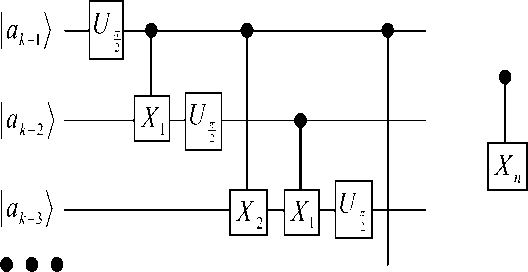
Figure 2. Circuit for QFFT of the variable | a k - 1. . a 1 a , J using Coppersmith s FFT approach. The two-bit

( 1	0	0	0   1
0	1	0	0
0	0	1	0
к 0	0	0	2 П /2 n e    7

“ X ” gate may itself be decomposed into one-bit and XOR gates

Suppose f (a) has period r so f (a + r) = f (a). The sum over a will yield constructive interference from the coefficients exp <

2 niac

. q

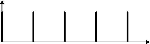
only when c is a multiple of the reciprocal period . All other values Qr of Qc will produce destructive interference to a greater or lesser extent. Thus, the probability distribution for finding the first register with various values is shown schematically by Fig. 3.

prob ( c )

3/ r

1/ r      2/ r

Figure 3. Plot of the probability of each result prob (c) versus c/q. Constructive interference produces narrow peaks of the inverse period of the sequence 1/r

c/q

One complete run of the quantum computation yields a random value of c/ q underneath one of the peaks in the probability of each result prob(c). That is, we obtain a random multiple of the inverse period. To r extract the period itself we need only repeat this quantum computation roughly log log times in order to k have a high probability for at least one of the multiplies to be relatively prime to the period r - uniquely determining it. Thus, this algorithm yields only a probabilistic result. Fortunately, we can make this probability as high as we like.

Quantum Computing: Unified Approach to Fast Unitary Transforms

Discrete orthogonal transforms and discrete unitary transforms have found various applications in signal, image, and video processing, in pattern recognition, in bio-computing, and in numerous other areas. Well-known examples of such transforms include the discrete Fourier transform (DFT), the Walsh-Hadamard transform, the trigonometric transforms such as the Sine and Cosine transform, the Hartley transform, and the Slant transform. All these different transforms find applications in signal and image processing, because the great variety of signal class, occurring in practice, cannot be handled by a single transform.

On a classical computer, the straightforward way to compute a discrete orthogonal transform of a signal vector of length N takes in general O(N ² ) operations. An important aspect in many applications is to achieve the best possible computational efficiency. The examples mentioned above allow an evaluation with as few as O(N log N) operations or – in the case of the wavelet transforms – even with as little as O(N) operations. In view of the trivial lower bound of Q ( N ) operations for matrix-vector-products, we notice that these algorithms are optimal or nearly optimal.

Remark : The rules of the game change dramatically when the ultimate limit of computational integration is approached, that is, when information is stored in single atoms, photons, or other quantum mechanical systems. The operation manipulating the state of such a computer have to follow the dictum of quantum mechanics. However, this is not necessarily a limitation.

A striking example of the potential speed-up of quantum computation has been given by Shor in 1994. He showed that integers can be factored in polynomial time on a quantum computer. In contrast, there are no polynomial time algorithms known for this problem on a classical computer. The quantum computing model does not provide a uniform speed-up for all computational tasks. In fact, there are a number of problems, which do not allow any speed-up at all. For instance, it can be shown that a quantum computer searching a sorted database will not have any advantage over a classical computer. On the other hand, if we use the classical algorithms on a quantum computer, then it will simply perform the calculation in a similar manner to a classical computer. In order for a quantum computer to show its superiority one needs to design new algorithms, which take advantage of quantum parallelism.

A quantum algorithm may be thought of as a discrete unitary transform, which is followed by some I/O operations. This observation partially explains why signal transforms play a dominant role in numerous quantum algorithms. Another reason is that it is often possible to find extremely efficient quantum algorithms for the discrete orthogonal transforms mentioned above. For instance, the discrete Fourier transform (DFT) of length N = 2 n can be implemented with O (log ² N ) operations on a quantum computer.

A quantum computer directly manipulates information stored in the state of quantum mechanical systems. The available operations have many attractive features but also underlie severe restrictions, which complicate the design of quantum algorithms. We are present a divide-and-conquer approach to the design of various quantum algorithms. The class of algorithm includes many transforms, which are well known in classical signal processing applications. We show how fast quantum algorithms can be derived for the DFT, the Walsh-Hadamard transform, the Slant transform, and the Hartley transform. All these algorithms use at most O (log ² N ) operations to transform a state vector of a quantum computer of length N .

Divide-and-Conquer methods. We have seen that a number of powerful operations are available on a quantum computer. Suppose that we want to implement a unitary or orthogonal transform U ∈ U (2 ⁿ ) on a quantum computer. The goal will be to find an implementation of U in terms of elementary quantum gates. Usually, our aim will be to find first a factorization of U in terms of sparse structured unitary matrices U , U ≅ U U U , where, of course, k should be small. It is often very easy to derive quantum circuits for structured sparse matrices. For example, if we can find an implementation with few multiply controlled unitary gates for each factor U , then the overall circuit will be extremely efficient.

Remark. The success of this method depends of course very much on the availability suitable factorization of U . However, in the case orthogonal transforms used in signal processing, there are typically numerous classical algorithms available, which provide the suitable factorizations. It should be noted that, in principle, an exponential number of gates might be needed to implement even a diagonal unitary matrix. Fortunately, we will see that most structured matrices occurring in practice have very efficient implementations.

In fact, we will see that all the transforms of size 2 n x 2 ⁿ discussed in the following can be implemented with merely O (log ² 2 ⁿ ) = O (n ² ) elementary quantum gates. We discuss a simple – but novel – approach to derive such efficient implementations. This approach is based on a divide-and-conquer technique. Assume that we want to implement a family of unitary transforms U , where N = 2 ⁿ denotes the length of the signal. Suppose further the family U can be recursively generated by a recursive circuit construction. We will give a generic construction for the family of pre-computation circuits Pre- and the family of post-computation circuits Post. This way, we obtain a fairly economic description of the algorithms.

Example: Assume that total of P ( N ) elementary operations are necessary to implement the precomputation circuit Pre . Then the overall number T ( N ) of elementary operations can be estimated from the recurrence equation T(N) = T(N/2) + P(N). The number of operations T(N) for the recursive implementation can be estimated as follows:

LEMMA : If P ( N ) e © ( log ^p N ) , then T ( N ) e O ( log p ^{+ 1} N ) .

Fourier transform . We will illustrate the general approach by way of some examples. The first example is the DFT. A quantum algorithm implementing this transform found a most famous application in Shor’s integer factorization algorithm.

Example: Algorithm and Physical Interpretation of Fast Fourier Transform (FFT). Consider a signal (any quantity that is a function of time, perhaps pressure in the air) affecting a system (anything that responds to a signal, like a microphone). The outcome of this interaction is called, naturally, the response of the system to the signal. The question is. How are we to compute such response digitally? In many applications (in which often the horizontal axis is not time, but also space, e. g. in image processing) it is of great interest to compute the system response, thereby simulating the system. The following is a rough description of how this is done.

First we digitize the signal, by sampling it often enough. Then we must know how the system behaves. It turns out that, if the system is time invariant (does not change its behavior over time) and linear (roughly, gives twice the response to twice the signal), then its behavior is completely captured by its impulse response - a description of what it does over time if it is given a sudden unit “jerk” at time zero. If we know that, since any signal is the sum of such jerks happening at various times, and since we know that the system is timeinvariant and linear, then all we have to do is calculate the responses at various times, and add them to get the total system response.

Remark : To do the algebra, suppose that the signal is the sequence ( a ,…, a ) of real numbers, and the system impulse response is ( b ,…, b ) (assume that they both have the same time horizon, that is, they both die after T time unit. Then at time 0 we have the system response a b - only the first pulse of the signal has arrived, and has only gotten the immediate response b . At time 1 we have the system response a b + a b , because now a gets the immediate response, while a causes the delay-1 response of the system, and the two are added. After two steps, then the system response is a b + a b + a b .

What is the system response after t time units? If t <  T, that is, if the signal keeps arriving at time t, then it is c _t = ^ abt-i . If t - T — that is, if the signal has died out — then the system response keeps coming, since the system keeps responding to the signal in the past: The system response is then c =

T / -t T+b^fF *" Finally, at t = 2T — 1 we have c 2r-2 = a_T_₃b_T -i, and thereafter c_t = 0: the system response has died out.

This sequence of formulas for c ,…,c     are precisely the formulas for the coefficients of the product of product of two polynomials.

/ t - 1       A

T aax

V       J

( T - 1

• T bx

V i = 0

2 T - 2

= T cx i=0

This is not a coincidence: We can think of both the signal and the system response as two polynomials in x, where x can be thought of as a unit delay, x ² two delays, etc. Then the product of the two polynomials is, naturally enough, the system response.

Conclusion: It is of great interest to compute very fast the coefficients c , t = 0,…, 2T – 2, of the product of two given polynomials of degree T - 1.

Unfortunately, just by looking at the formulas, the number of operations required to compute the c ’s seems to be Q ( T ² ): The number of terms increases from 1 to T and then down to 1 again, for a sum of about T ² . How can we calculate the c ’s much faster?

Remark: The c_t ’s are the coefficient of the polynomial C(x) = T -_₀ c_tx = A(x)B(x) , where A(x) = T._₀ ^a_tx^l , and B(x) = T■ -o b^ " And here is a scheme for calculating these coefficients:

1	Calculate the values of A(x) and B(x) at enough points x, ,^, xn where n >  2T -1.
2	Calculate the values of C(x) at these points as C(xJ = A ( x, ) • B ( x, ) , 1=1,^, n
3	Now that we know at least 2T - 1 values of the 2T - 2-degree polynomial C(x), we can interpolate and recover the coefficients. (Recall that there is a unique d-degree polynomial that goes through d+1 points.)

But there are problems with this approach: Although step (2) is easy (it only requires n multiplications), step (1) seems to still require Q (n ² ) operations, and step (3) seems even harder. Have we accomplished nothing with this clever manoeuvre?

It turns out that we need another trick: Pick the points x ,…, x on which to evaluate A(x) and B(x) so that the n evaluations can be done together very fast. It turns out that the most clever way to choose these points is to find n different points x ,…, x such that the equation x ⁿ = 1 holds for all of them.

Remark: Obviously, there are at most two real numbers that satisfy this equation: 1, if n is odd, and perhaps –1, if n is even. But there are exactly n complex numbers that do: The n complex roots of unity . They are n points lying, in the complex plane, on the unit circle. And since on the unit circle rising to the n th power means multiplying the angle by n , all n of these numbers are mapped to the real unity when raised to the n th power. Let us call then x ₁ = 1 , x ₂ = w, x₃ = w ² , x₄ = w ³ ,..., x _n = w ^{n - 1} . What we need to remember from now on about these numbers is that w is some number satisfying w ⁿ = 1 – nothing else. Except one thing: If we take a root of unity like w i , and add its powers 1+ w i +w ² i + ... +w ^{( n - 1)} i then we get 0 - because the powers of w ⁱ are just points around the origin, “pulling it in all different directions.” With one exception: If i = 0, then of course the sum is 1+1+…+1 = n .

We conclude that we want to find a fast way to compute these n values:

n - 1

A ( w i ) = T a^w¹ , j =0,—, n — 1.                                 (1)

i = 1

In this equation (1), j varies over 0,…, n – 1 to define the n points x ,…, x on which to evaluate A(x), and the summation is the value A( x ) = A( w ^j ). We need to remember all the time that w ⁿ = 1 – this is the fact that is going to save us from the Q ( n ² ) algorithm.

We are going to compute all n values in (1) together, by divide-and-conquer. Assume that n is a power of two – presumably the next power of two above 2 T – 2. Then, we divide the sequence of coefficients a₀ ,..., a_nl into two subsequences: The even subsequence a₀, a ₂ , a 4 ,..., a_n_,, and the odd subsequence a_x, a₃, a_s ,..., a _n4 . Then we can write (1) as

A( w j )	=	n - 1                n - 1 22 Y a3iw 2 iJ + V a 2/+i W 2 ' + ' 2 i                         2 I + 1 i = 0                   i = 0
	=	n - 1                        n -1 22 Z a 2 i ( w 2 ) ij + w J Z a 2 i +1( w 2 ) i J i = 0

Now this equation is just two problems of the same kind applied to sequences of length n (compute the values of a degree n - 1 – polynomial at the n -nd roots of 1 – notice that is 1, w 2 , w 4

2 n - 2

w    are

precisely the ⁿ -nd roots of unity). To obtain the A( w ^j ) from the results of the conquered subproblems, we just multiply the j mod ⁿ -th result of the second evaluation by w ^j and add it to the corresponding j mod ⁿ -th result of the first. The points on which we need to evaluate the subproblems are just ⁿ , because this is 22 the number of the possible values of ( w ² ) ^j . This is quintessential divide-and-conquer, with recurrence

T(n)

=

2T( n ) + n 2

Here the O(n) term is the work required to “put together” the results of the conquered parts ( n multiplications and additions). The total complexity of the algorithm is, as we know, O(n log n) .

Remark: This algorithm, which computes the values of an n -degree polynomial at the n n- th roots of unity in O(n log n) time by divide-and-conquer is called the Fast Fourier Transform (FFT). It is perhaps one of the most important and widely used algorithms; it was discovered by Cooley and Tuckey in the 1950’s.

Example: Notice that the FFT, as described so far, only takes care of Step 1 of this scheme: Evaluating A(x) and B(x) at n points. How are we to carry out Step (3) – recovering the coefficients of C(x) from these n values? The amazing fact is that this can be can be done with another FFT - but this time w ^{- 1} playing the role of w .

This is just algebra. Suppose that we apply this “inverse” FFT to the values of C(w j ), j= 1 ,...,n - 1,

n -1 Z C ( w J ) w -Jk j =0	=	n -1    n -1 Z ( Z c . wU) w k J =0   i =0
	=	n -1 Z i =0	n -1 Z cw' ( i - k ) L j =0            J

Consider however the inner sum of the last line, for some fixed values of i and k. If these values are the same, then the parenthesis contributes n. If they are not, then the powers of w i-k # 1 cancel each other. So, just ∑nj=-10 C(w j)w- jk=ck steps of polynomial multiplication algorithm now are these:

Step1: Compute the FFT of a ,…,a   top obtain the sequence A ,…,A   . Repeat with b ,…,b   top obtain the sequence B ,…,B   . Step2: Compute C := A ⋅ B , i = 0,…, n – 1 (note that these are complex number multiplications.) Step3: Compute the inverse FFT (FFT with w -1 in the place of w), and then divide the results by n, to obtain cn,..., c .. ,             0,,  n—1 the above sum is

- it recovers the coefficients of C(x) . To summarize, the three

Remark: We often need to solve the system response problem when the input signal is periodic – that is, it is repeated after n time units. The system response then is found by an FFT with half the points ( n = T ).

Remark: Also, since all we needed from w is the equations w ⁿ = 1 and

∑ wⁱ = 0 , we could use any

arithmetical domain where these equations hold – not necessarily the complex numbers with their slow multiplications. We shall see in good time that there are domains in which we are computing modulo a large integer, in which such equations hold.

Example: The FFT Circuit . As with all divide-and-conquer algorithms, it is worthwhile to unravel the recursion, to see what the algorithm really does. If we do this, the algorithm becomes the circuit shown in Fig. 4.

Remark: A word of explanation: The nodes are complex variables. The nodes on the left are the inputs (but in a funny order), and those on the right are the outputs. An arrow labeled with the integer j (unlabeled arrows are labeled “0”) from x to y can be though of as carrying the value xw ^j to y . The two arrows coming into a node (other than the input nodes) are added together. Under this interpretation, Figure 4 shows the FFT of eight points.

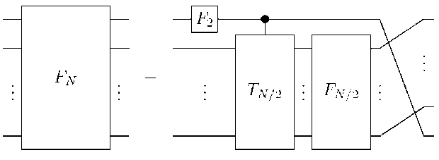
Figure 4. The recursive structure of the quantum Fourier transform

Notice these properties of this circuit:

•	There are 3 = log n levels, with n variables each, and four complex operations per variable (actually, seven real operations), for a total of 7 n log n operations.
•	There is a unique path between every input node and every output node.
•	The path between a and A(w j ) has label sum equal to ij modulo 8 (and it makes sense to take powers of w modulo 8, since we know that w 8 = 1).
•	The previous two facts ensure that the circuit correctly computes the FFT.
•	The inputs are mixed up this weird order. (Compare the binary representations of the indices of an input and an output that are opposite one another).
•	Notice how neatly arranged this circuit is for parallel evaluation. Indeed, the FFT is a natural for parallelism, and can be carried out in log n short parallel stages. Often the FFT is computed by specialized embedded parallel hardware.

•	Each stage of the FFT consists of n “ butterfly ” operations – a typical butterfly is the subcircuit shown in bold in Fig. 4.

Recall that the DFT F of length N = 2 ⁿ can be described by the matrix

= N	1     , ПТ" ( to     ) j , k =0,..., N -1' N

Where to denotes a primitive N- th root of unity, to = exp(2 n i / N) . And i denotes a square root of-1.

Remark: The main observation behind the fast quantum algorithm dates at least back to work by Danielson and Lanczos in 1942 (and is implicitly contained in numerous earlier works). They noticed that the matrix F might be written as

F N	=	P N	( F F N /2	F F N /2
			FT, V1 N/21 N /2	-F , T , 1 N/21 N /2 У

Where P denotes the permutation of rows given by P bx = xb with x an n – 1-bit integer, and b a single bit, and TNI1 :=diag(1, to , to 2 ,..., to N/2 1) denotes the matrix of twiddle factors.

This observation allows to represent F by the following product of matrices:

F = P

F _N = _N ^^

'7'    0 'V 0    FN/2 J

( 1

¹ N /2

V 0

1 ⁰ 1 F

N /2 у 2

¹ N /2    ¹ N /2

¹N /2      ¹N /2 J

Г1М„ 0 1,

= P N (1 ₂ ® F N, /2 )   " '2          ( F , ® 1 N ,2 )

V ⁰     T N /2 У

This factorization yields an outline of an implementation on a quantum computer.

Remark: It remains to detail the different steps in this implementation. The first step is a single qubit operation, implementing a butterfly structure. The next step is slightly more complicated. We observe that T _N/2 is a tensor product of diagonal matrices D. = diag(1, to ²   ). Indeed, T _N/2 = D _n_ , ® ... ® D ₂ ® D p

Thus, 1 _N/2 Ф T_V2 can be realized by controlled phase shift operations (see Fig. 5 for an example).

We then recurse to implement the FT of smaller size. The final permutation implements the cyrlic rotation of the quantum wires.

Example: The complexity of the QFT can be estimated as follows. If we denote by R(N) the number of gates necessary to implement the DFT of length N = 2 ⁿ on a quantum computer, then implies the recurrence relation R(N) = R(N/2) + 0 (log N ), which leads to the estimate R(N) = O (log ² N).

It should be noted that all permutations P_N (1₂ ® P _{N /2})...(1 _N__г Ф P ₄ ) at the end can be combined into a single permutation of quantum wires.

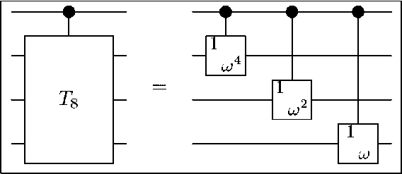
Figure 5. Implementation of the twiddle matrix 1₈ Ф T_&

The resulting permutation is the bit reversal, see Fig. 6.

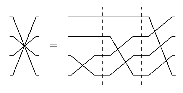
Figure 6. The bit reversal permutation resulting from p (1₂ ® p )(1₄ ® p )

The Walsh – Hadamar transform

Example: The Walsh-Hadamard transform W is maybe the simplest instance of the recursive approach. This transform is defined by the Hadamard gates W = H in the case of signals of length 2. For signals of larger length, the transform is defined by W = (1 ⊗ W )( H ⊗ 1 ).

This yields the recursive implementation shown in Fig. 7.

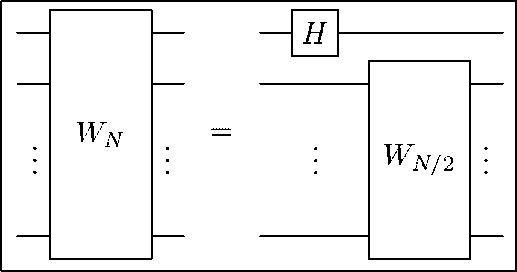
Figure 7. Recursive implementation of the Walsh-Hadamard transform

Since P(N) = Θ (1), the Lemma 3 shows that the number of operations T(N) ∈ O (log N ). It is of course trivial to see that in this case exactly log N operations are needed.

The Slant transform

Example: The Slant transform is used in image processing for the representation of images with many constant or uniformly changing gray levels.

Remark: The transform has good energy compaction properties. It is used in Intel’s ‘Indeo’ video compression and in numerous still image compression algorithms.

The slant transform S is defined for signals of length N = 2 by the Hadamard matrix

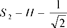
[1 Д ] к1 17

and for signals of length N = 2 ^k , N >2, by

S _N = Q _N

^S N /2

o

V^V N /2

0 N/2

S N /2 7

where 0 denotes the all-zero matrix, and Q is given by the matrix product

Q N = P N (1 N /2 Ф Q N )( H ® 1 N /2 ) P N ■

The matrices in (3) are defined as follows: 1 is the identity matrix, H is the Hadamard matrix, and

P ^a realizes the transposition (1, N /2), that is,

PaN 1 = N /2 PaN N /2 = 1 and P a x = x otherwise. easy to check that A is a unitary matrix.

Remark: The definition of the Slant transform suggests the following implementation. Equation (2) tells us that the input signal of a Slant transform of length N is first processed by two Slant transforms of size N/2 , followed by a circuit implementing Q . We can write equation (2) in the form

$ N = Q N 72  7'2   = Q N ( 1 2 ® S n /2 ) .

к ⁰ N /2 S N /2 7

The tensor product structure 1₂ ® S^^ is compatible with our decomposition into quantum bits. This means that a single copy of the circuit S acting on the lower significant bits will realize this part. It remains to give an implementation for Q . Equation (3) describes as a product of for sparse matrices, which are easy to implement. Indeed, the matrix P ^b is realized by conditionally excerting the phase gate Z . The matrix H ® 1_V2 is implemented by a Hadamard gate H acting on the most significant bit. A conditional application of A _v implements the matrix 1 _{N /2} ® Q)_N . A conditional swap of the least and the most significant qubit realizes P ^a , that is, three multiply controlled NOT gates implement P ^a .

THEOREM: The Slant transform of length N = 2 ^k can be realized on a quantum computer with at most O( log ² N) elementary operations (that is, controlled NOT gates and single qubit gates), assuming that additional workbits are available.

Proof. Recall that a multiplied controlled gate can be expressed with at most O(log N ) elementary operations as long as additional workbits are available. It follows from the Lemma that at most O (log ² N ) elementary operations are needed to implement the Slant transform.

The quantum circuit realizing this implementation is depicted in Fig. 8.

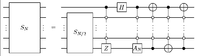
Figure 8. Implementation of the Slant transform

The matrix P ^b is defined by P ^b x = x for all x

except in the case x= N/2+1, where it yields the

phase change P b_N | N /2 + 1 = - | N /2 + 1. Finally Q_N =

[ AN

1,„

AN

a and b are recursively defined by a = 1 and b

к

J1 + 4 ( a ,/2 ) 2

and

[-7

к ^N

aN

bN ) aN 7

, where

2b _N a_{N /2} . It is

The recursive step is realized by a single Slant transform of size S . The next three gates implement p , H ®1_№2, and 1y/2 ® Qn , respectively. The last three gates implement P ^ . Thus, the implementation of Q totals five multiply controlled gates and one single qubit gate.

The Hartley transform

Example: the discrete Hartley transform H is defined for signals of length N=2 ⁿ by the matrix

^HN =  ^ ( cos^ l ) + sin ( ^{2 n kl} )) _k , I = 0.., N -, .

Remark: The discrete Hartley transform is very popular in classical signal processing, since it requires only real arithmetic but has similar properties. In particular, there are classical algorithms available, which outperform the FFT algorithms. We derive a fast quantum algorithm for this transform, again based on a recursive divide-and-conquer algorithm. A fast algorithm for the discrete Hartley transform based on a completely different approach has been discussed by Klappenecker and Rotteler.

The Hartley transform can be recursively represented as

HN

f 1

1 ,»

V ¹ N/2

¹ N ^/2 T ¹

¹ N /2 JV

V n

H N /2

BC N /2 Jv

H N /2 J

Q N ,

where Q N is the permutation Q N | xb = | bx^, with b a single bit, separating the even indexed samples and the odd indexed samples; for instance Q 8 (x0, x,, x2, x3, x4, x5, x6, x7)t = (x0, x2, x4, x6, x,, x3, x5, x7)t.

The matrix BC is given by

^BCN /2

f 1

V     ^CSN /2-1 j

with

c N

¹ s_N

N/4-1

cNs

N / 4 -1               N / 4-1

sN

V s N

cN J

The equation (4) leads to the implementation sketched in Fig. 9.

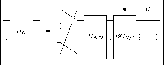
Figure 9. Recursive implementation of the Hartley transform.

Remark: It remains to describe the implementation of BC . It will be instructive to detail the action of the matrix ВСшг on a state vector of n -1 qubits. We will need a few notations first. Denote by |bx^ a state vector of n -1 qubits, where b denotes a single bit and x an n - 2 bit integer. We denote by x' the two’s complement of x. We mean by x = 0 the number 0 and by1 the number 22n-2 — 1, that is, 1 has all bits set and 0 has no bit set. Then the action of BC on bx is given by

BCN/2 00 = 00 , BCN /2 0 V)  =  cN \0 y)+sN i y'}, BCN /2 01)  = 01 , BCN/2 1 y)  =  sN' 0 y -c cN' 1y , where sk = sin (2nk I N) and ck = cos(2nk / N).

We are now in the position to describe the implementations of BC shown in Fig. 10. In the first step, the least n - 2 qubits are conditionally mapped to their two’s complement. More precisely, the input signal | bx is mapped to | bx ') if b =1, and does not change otherwise. Thus, the circuit TC implements the involuntary permutation corresponding to the two’s complement operation. This can be done with O ( n ) elementary gates, provided that sufficient workspace is available. In the next step, a sign change is done if b - 1, that is, |1 x^ ^ -| 1 x ^ , unless the input x was equal to zero, 110) ^ |10). The next step is a conditioned cascade of rotations. The least significant bits determine the angle of the rotation on the ( n - 1 st ) most significant qubit. The k- th qubits exerts a rotation,

R

2 ^k

fcos(2n2k 1N)- sn(2n2k 1N)) ( sin (2n2k I N) cos(2n2k IN) J on the most significant qubit. Finally, another two’s complement circuit traditionally applied to the state.

One readily

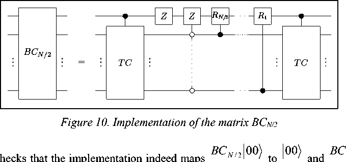
^{N /2 10} to ¹⁰

.

0 x              c 0 x) + s 1 x                                     1 x f he input      is mapped to N        N     , as desired. Assume that the input is     with x ^ 0 . f hen the state is changed to |1 x ^ by the circuit TC, and after that its sign is changed, which yields -|1 x '^. The rotations map this state to sx′ I 0x′ - cNx′ I 1x ′ . The final conditional two’s complement operation yields the state s x′ I 0x′ - cNx I 1x , which is exactly what we want.

The initial permutation, the circuit BC and the Hartley gate in Fig. 9 can be implemented with Θ (log ² N ) elementary gates. It is crucial that additional work bits are available, otherwise the complexity will increase to Θ (log ² N ). The Lemma completes the proof of the following theorem:

THEOREM : There exists a recursive implementation of the discrete Hartley transform H on a quantum computer with O (log ² N ) elementary gates (that is, controlled NOT gates and single qubit gates), assuming that additional work bits are available.

It should be emphasized that the divide-and-conquer approach is completely general. It can be applied to a much larger class of circuits, and is of course not restricted to signal processing applications. Moreover, it should be emphasized that many variations of this method are possible.

The method of the design of quantum algorithms takes advantage of a divide-and-conquer approach [118]. We have illustrated the method in the design of quantum algorithms for the Fourier, Walsh, Slant and Hartley transforms. The same method can be applied to derive fast algorithms for various discrete Cosine transforms. One reason might be that the quantum circuit model implements only straight-line programs. We defined recursions on top of that model, similar to macro expansions in many classical programming languages. The benefit is that many circuits can be specified in a very lucid way.