Structure design toolkit of quantum algorithms. Pt 3

Let us consider the description of Quantum Fourier Transform (QFT). The universality of the QFT in forming the basis of quantum computing algorithms is considered. The unique universal fundamental properties of quantum computing concerning quantum superposition, entanglement and interference are all explicitly represented in terms of quantum multiparticle interferometry [1-18].

The Universality of the Quantum Fourier Transform in Forming the Basis of Quantum Computing Algorithms

The Quantum Fourier Transform (QFT) on the additive group of integers modulo 2 ^m is defined by.

^F 2 " (I a) )

2 " -1

For a e { 0,1,2,...,2 " — 1 } .

/ . ■ ) /2 » ,  (1)

y =0

QFT plays a significant role in the development of the quantum computer (QC). One may note, for example, that the potentially powerful integer factoring algorithm by P. Shor relies critically on the QFT for the detection of periodicity springing from the prime factors.

We can further analyze (1) as follows. First, write a = a12" 1 + a2 2" 2 + —+ a—-121 + a— 20 = (a1 a2 .a—)

2 ——1 ।      — ——2 .      .           1 ।      о 0    /                 \ anu          + ’ 22   + — + ’——12 + ’— 2 = ( y 1 y 2 — y— )

Then it is well known that

RHS of (1)	=	2 " — 1 E e ( 2'""2 " *1 ’ 1 — ’ —) y = 0
	=	2 " — 1 V^1  2 n "( 0. a — ) y 1 I    \  2 n (0. a — — 1 a — ) y 2|     \ .    2 n (0. a 1 a 2 — a — ) y — I      \ /v e           |y 1 / e               |y 2/    e                 |y—/ y = 0
	=	( 0^ + e 2n ( 0. a " ) 1 ^)( 0^ + e 2n ( 0. a " — 1 a " )| 1) )— ( 0^ + e2n ( 0. a 1 a 2 — a — ) 1 )

In the above factorization (or “untangling”), each factor is of the form |0^ + e^№\ 1 .

Remark: Such a state can be produced in two steps:

First, apply the transformation H = ,                     V21

— 1

where H is known as the Walsh-Hadamard trans-

form, to the state 1^0: H 0) = ^(10)+11)).

elto

, yielding P( to ) [ H |0^] = -^= ( 0^ + e™ |1 )

Remark: The RHSs are equal (apart from a normalization coefficient). Therefore, we see that the constituents of the QFT are H and P ( to ) . From the quantum optics point of view, H is realized by a halfsilvered mirror (beam splitter) and P ( to) represents a phase shifter, as in a standard Mach-Zehnder interferometer.

First, we wish to emphasize that the QFT strictly by itself is not universal in quantum computing (see Remark below). Thus, the question becomes whether the two constituents H and P ( • ) of QFT are universal or not. We will discuss the following problem:

“ Any QC algorithm can be represented as a composition of Walsh-Hadamard transforms and associated conditional phase shifts .”

Remark: The implication of this problem is that the realization of any QC algorithm translates into a combination of elementary quantum interferometric operations, i.e., single particle beam splitter (Walsh-Hadamard transform) followed by a conditional phase shift. Any QC algorithm can thus be formulated, or reformulated, in terms of elementary multiparticle quantum interferometric operations. The unique universal fundamental properties of QC concerning quantum superposition, entanglement and interference are all explicitly represented in terms of quantum multiparticle interferometry (QMI).

Remark . QMI practically is not to be taken as a proposed embodiment of a QC any more than the Turing machine is to be taken as a literal construction in classical computing. Rather, Ekert has suggested its equivalence to QC in the sense of its universality, meaning that QMI could be viewed as the closest QC analogue of the classical Turning machine (through the universality theorem established in this appendix). This concept and viewpoint should provide physical insights into the operational aspects and can facilitate efficient design of a universal QC.

Mathematical proof of the Universality of H and P(.)

As usual, we let U ( n ) to denote the unitary group on n-dimensional space. By abuse of notation, we regard ^{U ( n} ) the same as the multiplicative group of all n x n orthogonal matrices.

SO ( n ) denotes the orthogonal group on n -dimensional spaces or, equally, the multiplicative group of all n x n orthogonal matrices. We also define the maximal tours T ( n ) in U ( n ) as

T(n) = {d lag(elto,...,eto")|toto,...,to G^} , i.e., T(n) consists of all n x n diagonal matrices whose diagonal entries are complex numbers of unit magnitude. T (n) is a subgroup of the multiplicative group U(n ).

Let A be a collection of n x n unitary matrices. We will use gn (A) to denote the unitary subgroup of U(n) generated by A, i.e., gn (A) = flG \G«is a subgroup of U(n), A c Ga} a

We will write g_n ( A ) simply as g ( A ) if the value of n is clear from the context.

We begin with n = 2 .

Lemma: We have U (2 ) = g (SO (2), T (2)) , i.e., U (2) is generated by SO (2) and T (2); more precisely, for every A e U (2), we have ee/2     01

0     e -""= ^,

A =

e ^

e ^{a /2}

cos to

sin to

e i '⁵

e ^{a /2}

- sin to

costo

for some ^a , ^в , 8 , ю ^ ^

Lemma : T ( 2 ) c g ( H , P ( • ) ) .

Proof. We first note that the NOT-gate X =

can be obtained as

X = HP (- n)H.

Therefore X E g ( H , P ( • ) ) . From this, we have

XP (® )XP (®2 ) =

1    1

0 0

e1®1

0 110

1  0 0   e ®

e ®   0

0   e ®

for any given ® , ® E R. Therefore g ( H , P ( • ) ) contains the maximal torus T ( 2 ).

Lemma SO ( ² )_E g ( ^H , ^P ( • ) ) .

Proof. For each rotation matrix cos® sin ® - sin ® cos® , we easily verify that

R (®) = PI п I HP (®)XP (- ®)HP I - n

g ( H, P (•)) = U ( 2 ).

Theorem:

Proof. This follows immediately from Lemmas.

Decomposition Procedure of General Finite Dimensional Unitary Transformations into a Product of Plane Unitary Transformations

TpДф^Е U(n) by T Дф^)=[^J  , pq                          pq           j nXn

First, we define a special type of unitary transformations

1 <  p , q <  n , p ^ q , where

tj = 1

cos ф ,

0,

- e -^a sin ф ,

e ^ш sin ф ,

г = j,* ^ p j ^ q ,

* = j = p or *' = j = q , г ^ j,* ^ p , j ^ q and i ^ q , j ^ p , i = p and j = q , i = q and j = p ;

p

q

с     г

1  0  0

0   1

^Tpq ^(ф , " ) =

cosф - e " sin ф e" sin ф     cosф so

	- * •
t L V =	: *
n , n - 1	L u n 1

*

*

'

^U n , n -1

^U 1 n

'

^U n -2, n

T_p фф,"' ) is just a plane unitary transformation acting non-travially only on states p and q .

Let V e U ( n ).	We want to find some T n , n	_ 1 ( ф , " ) such that T n * n_X V = V ‘		U ■ 1 n X n	where и	n - 1, n    0
	"10 0	1
	0  1   0		" U 11      •	•     U 1, n - 1	U 1 n "
	0  0   1	0	i		:
T n , n- V =						’
	4		U n - 1,1     •	• и , n - 1, n -	U n - 1, n
	cos ф	e - i " sin ф	L U n 1      •	U n , n - 1	U nn _
	0       - e i " sin	ф       cos ф

^U n - 1, n = ^U n - 1, n ^{cos ф} + ^U nn e "  ^{sin ф} -

We consider all possibilities:

Case 1:	U i = 0. Then we choose ф = 0, " = 0, i.e., T _j n ( ф , " ) = I , and we obtain U n - 1, n = U n - 1, n = 0.
Case 2:	U„i „ ^ 0, u = 0. Then choose ф = n /2, " = 0. Obtain U  „ = 0. n 1, n           nn                                                                             , n
Case 3:	U л ^0,0  ^ 0. Write U , =r , (г6"1 -1, n, U —r el9nn . Choose n -1, n       , nn                      n - 1, n      n - 1, n          ,    nn      nn       . " = - 6 n -1, n + 6 nn and ф = tan - 1 ( - r n - 1, n / r nn )• Obtain U n - 1, n = cos ^ r n - 1, n e6" - 1, n + sin ф - r nn el ( - " + 6nn ) ( r A =      , + tan ф r „cos ф e n 1, n = 0. nn V r nn            /

Therefore, we have found T_{n n 4} e U ( n ) such that

Similarly, we can find T _₂, T _ _W - T T _x such that n ,,,

*

*

''

т * Л* У = n , n — 2 n , n —г

^U n — 3, n

*

''

^U n 1

*

''

^U n , n — 1

''

^U nn

*

*

T * T* T* T* v = n 1 n 2 ^— n , n — 2 n , n — 1

= W.

*

*

и

~ n, n—1

~nn

~   ~

Since W is unitary, we conclude   ^{n 1     n1}

~

^U n , n —1

= 0

~ and nn

= ea = d        a e R.

ⁿ for some ⁿ     Thus

T *T*   T* T* y = n 1 n 2“ У, n—2 n, n—Г

**

.

dn

Now, applying the same technique to the remaining ( n — 1 ) x ( n — 1 ) undiagonalized matrix block ( ** )

above, together with a simple induction argument, we obtain plane unitary transformation

T. 1,-,Tn,, —,.Tn—1,1,-,T.—1,—2,-,Тз„T32 and T:] such that d 1

*  *  .   *      .         *     „      .

T 21 T 31 T 32 T 41 ^— T n — 1,1 ^— T n — 1, n — 2 T n 1 ^— T n , n — 1 V

d 2

= D,

where d _y = e ^a for j = 1,2, - , n .

Therefore

V^T T    T T     T   T T T D y       n , n —1,^ n , n —2 - -± n 1^ n — 1, n —2 - -± n —1,1 - -± 32-l31±211v
=	(  n   i — 1 ПП T,, \ i = 1   j = 1       J	D .

At this point, it should already be clear that U ( 2 ⁿ ) can be generated through controlled-U (2) gates , for any n = 1,2,^. Let us give the following concise, rigorous treatment as to how to construct any V e U ( 2 ⁿ )

from a serial connection of a collection of unitary matrices V_tJ, where each V y is a (generalized) controlled- U (2) gate. The precise statement is given below.

Theorem: Let V e U ( 2 ⁿ ) Then

2 ⁿ — 1 i — 1

V = ПП Vj.

i = 1 j = 0

For a collection of matrices Vy e U ( 2 ⁿ ) such that

V ₇:   Sy ^ Sy  is the identity transformation ,

S_ti = span

{ m^|m e{0,1,.2n -1}, m * i, m * j }  >

0 < j < i < 2n -1.

In other words, each V e U ( 2 ⁿ ) is a product of (generalized) controlled-U(2) unitary matrices J f, which acts nontrivially only on S ^ = span { i ^ ,| j }

Proof. We first quote the following fact (see above). For any V e U ( 2 ⁿ ) , there exists a collection of

(2 n - 1 i - 1      7

V = ПП T. , j D ,

unitary matrices T y ,0 < j < i < 2 ” -1, and a D e T(2n ) such that к i=1 j=0     7

where T_t>J e SO ( 2 ⁿ ) c U ( 2 ⁿ ) is a rotation involving i and j and satisfying the above mentioned condition. Now we can break up D into

A

(a d 0

D =

' ^d 0

к

d ₁

where D_x =

к

d ₁

= D 1 D 2 . D 2 n - 1

d d 2n -17

A

and D_i =

d _i

A

17

к

17

for i = 2,3, . ,2 ” - 1. It is easy to see that D_v acts trivially except on

0 and 1 , and the other D ’s act

non-trivially only on

addition, D ’s commute with each other, and each D commutes with

T_k /, V 0 <  l <  k <  i as well.

Thus,

y = T

2 ⁿ - 1,2

n

...T T

-2 .  2 n - 1,0  2 n - 2,2 n

...T

3 . 2"

T T T D D D .2,0 ■■■ T 2,1 T 2,0 T 1,0 ^D 1 ^D 2 ■■■^D ₂ n - 1

= T    T

2 ⁿ - 1,2 ⁿ - 2  2 ⁿ - 2,2 ⁿ

T

- 3           2'

n

- 1,0

.^D 2 n - 1

T       ... T

2 n - 2,2 n - 3       2"

- 2,0 ^D 2 n - 2

^ 2n -1

T T D

2,1  2,0   2

T D

1,0    1

strings of products. For 0 < j < i < 2n -1, define ij

T i, j

T D = T D i, j     i          i ,0 i

if j * 0, if j = 0.

2 n - 1 i - 1

Therefore we have reached V = ^^ ^^ V, , where each V^ is a unitary matrix which acts nontrivially i = 1 j = 0

only on the states i and j satisfying the above mentioned expression.

Remark. The factoring of D into the product of D_v , D^ ,... and D _f in the presented forms is peculiar in the sense that D 1 is chosen differently from the other D _z ’s, i ^ 1. It must be done this way. The reason for this is that there are 2 n — 1 strings of products as indicated above. Therefore D must be factorized to have 2 n — 1 factors D_x , D ₂,..., D^n , in the unique way.

Remark. Now it can be readily seen that the QFT itself is not universal in the sense that U(2n ) is not generated by F (cf., with case m = n therein) or (generalized) controlled- F^m (where m < n ) operations. First, check n = 1: we see that F = F2 is actually the Walsh-Hadamard transform H (apart from the normalization factor 1/V2 ). Therefore, the phase shifts P(to) in (2) cannot be generated by F2 because P(to) has eignevalues 1 and eto while H has eignevalues 1 and -1. For a general positive integer n, the range of F or of controlled- F^m, m < n, consists at most of linear combinations of states of the form e 2^[(0. a) y 1 +(0. an—1 an) y 2+-+(0. a 1^ an) у, ]

|У 1 -• У п \ where a_} , y_} e { 0,1 ), for j = 1,2,..., n .

The phases of such states are not even dense with respect to all possible phases e^{2m e} , 0 <  0 <  2 n .

Remarks on Circuits . The decomposition (3) is a mathematical rendering of above mentioned statement and answers the conjecture affirmatively.

Each factor V_y in (3) satisfies (4) and thus V_y acts nontrivially only on the states | z ) and | j ^. Denote

A

the restriction of Vy to the 2-dimensional subspace q^ = span {| z) ,| j^} by V^. Then Vy e U(2). Each Vy is not a standard Ли1 ( V ) gate is the sense that the controls are states rather than bits.

Nevertheless, point out how to rearrange basis states with a “gray code connecting state i to state I j ” such that V_y becomes unitarily equivalent to Л_и1 ( V ) . In this sense, V_y are generalized controlled- V gates.

Proposition. The symmetric group S n of permutations on the symbols 0,1,2,…,2 ⁿ -1 is generated by the 2-cycle ( 2 ⁿ — 2,2 ⁿ — 1 ) and the 2 ⁿ - cycle ( 0,1,2,...,2 ⁿ — 1)

Proof. This is a basic fact of group theory.

Incidentally, we note that the 2-cycle ( 2 ⁿ — 2,2 ⁿ — 1 )

is a permutation between the states

11 ^ 10

n bits

and

11.. .1 ) and thus can be realized by the controlled-NOT gate with the n th qubit as the target bit and the first '-------V------- '

n bits

( n — 1 ) bits as the control bits as shown in Fig. 1.

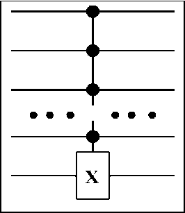
Figure 1: The n -bit controlled-NOT gate

On the other hand, the 2 n -cycle    ^{( o,1,2,}•••^,2   1 )   makes

10) ^И) ^ --I2n —2) ^|2n —1 ^|01         lx) ^ x +1 mod 2n i.e., the mented by the circuit as shown in Fig. 2.

the rotation of the states operation. This can be imple-

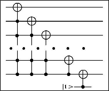
Figure 2. This circuit implements the operation |x ) ^| x + 1mod2 ⁿ) or, equivalently, the 2" -cycle (0, 1, 2, . . . , 2 ⁿ . 1) in Proposition. Note that the bit 1 at the bottom of the figure is the “scratch bit” which is sometimes omitted in circuit drawing. All the gates in this circuit are controlled-NOT gates

Therefore, any permutation of the basis states | x ), x = 0,1,2, .„,2 ⁿ — 1, can be realized by finitely many

controlled-NOT operations consisting of circuits as shown in Figs 1 and 2.

Thus, each factor V in (2) can be realized by the circuit as shown in Fig. 3.

	(i,2° - I) (j,2n -2)
• •		J

	<л2П-1) (j,2n -2)
L		• •
IJ

Figure 3: The unitary matrix V.. as a controlled- V.. gate where V g U (2) . The operations ij                                           ij                                 ij

( i ,2 ⁿ — 2 ) and

j, 2n . 2) in the two boxes are cyclic permutations (which can be realized by concatenations of circuits in Figs 2 and 3

By concatenating together all the blocks V as shown in Fig. 2 according to the factorization (2), we have constructed all V e U ( 2 n ) with controlled- V_tj gates according to (2). Each V e U ( 2 n ) is then further formed from concatenations of the gates H , P ( ® ) e U ( 2 ) according to corresponding Theorem. It is in this sense that we have the universality of the Walsh-Hadamard gate H and the phase shift gate P ( • ) and, consequently, that of the QFT with the affirmative answer to the above question.

Example : Another Way to Perform the Quantum Fourier Transform in Linear Parallel Time . Shor’s factoring algorithm suggests that quantum computers can do things in polynomial time that classical computers cannot. However, since decoherence due to storage errors is a function of time, we should also ask to what extent we can parallelize quantum algorithms; if we can do many quantum operations at once, rather than serially, we can solve larger problems before our computer decoherens.

Consider a quantum circuit operating on a set of qubits, containing one-qubit gates (2 x 2 unitary matrices) and the two-qubit controlled-not-gate; these are universal for quantum computation. We can define the depth of this circuit as the number of layers, where each layer consists of gates operating on mutually disjoint sets of qubits; that is, each qubit interacts with at most one other qubit at time. (In a model of quantum computation where one qubit can simultaneously interact with several others, we could allow gates operating on the same qubit in the same level, as long as these gates all mutually commute.)

The heart of Shor’s algorithm is the Quantum Fourier Transform. If we represent n -digit numbers a

2 n - 1

with n qubits, the QFT maps | a ^ to 2 ^{- n}/2 ^ e^{2 m ab /2} b .

b = 0

We exhibit a circuit with depth O ( n ) for performing the QFT.

Griffiths and Niu have already done this, in fact in a more natural way.

We exhibit a quantum circuit that performs the QFT on n qubits in O ( n ) depth. Thus, a parallel quantum computer can carry out the QFT in linear time. Griffiths and Niu have already shown this. We also speculate as to whether the QFT might be in the class QNC of problems solvable in logarithmic parallel time.

The standard quantum algorithm for the QFT takes n ( n - 1 ) /2 gates. One way to construct it is to reshuffle the rows of the matrix by putting the digits of the input in reverse order. Then for n =3, for instance, we have

Г1 1 1 1 1 1 1 1   ) 1 -1 1 -1 1 -1 1 -1 1 z -1 -i 1 i -1 -i 1 -z -1 i 1 -i -1 i 1 em/4 i 3ni / 4 -1 5п/4 -i 7 ni/4 1 5п/4 i 7П/4 -1 en/4 -i e3n/4 1 3ni / 4 - i en/4 -1 7n/4 i 5ni/4 b 7 ni /4 e - i 5ni /4 e -1 3ni /4 e i m /4 e   V where we are suppressing a factor of 2 3/2.

If we call this F (3), we immediately notice that its upper-left and upper-right quadrants are

П 1 1 11 1 -1 1 -1 1 i -1 - i .1 - i -1 i V which is simply F(2). The lower-left and lower-right quadrants of F(3) are F(2) and –F(2), with a series of phase shifts applied to the columns; this can be expressed by multiplying on the right by the matrix

A

( 1

e

П /4

i

V

3 П /4

e 7

which we will call M . In general, we can write

F ( n + 1 )	=	1 2	( F    F 1 V FM - FM 7
	=	( F  ^)'	( 1     1- т ( 1   1 1 v    m 7 V2 V 1 - 17

We recognize this as the circuit for F(n) applied to the n least significant qubits, followed by a gate where the most significant qubit controls whether or not to apply the phase shifts M , followed by the

„    1 ( 1   1 1

applied to the most significant qubit.

Hadamard operator H = -i=

V 2 V 1   - 1 7

Finally, note that M is simply a tensor product of independent one-qubit operations

M =

V

1i 7

®

n il 4

e 7

®

A

e ^{n 18}

® • ••

Then the controlled- M gate becomes a series

(1

7

of controlled phase-shift gates

1   (1

A

(1     1

V M 7

®

i 7 V

n il 4 e

® •■•

These gates are symmetric, in that the “controlled” and “controlling” qubits are interchangeable. Putting all this together gives us the recursive construction.

To what extent can this circuit be parallelized?

Even though all the phase shift gates within a given pair of H ’s commute with each other, we can’t perform them simultaneously unless we can couple one qubit to multiple qubits at the same time, and they don’t commute with the H preceding them. Thus, it would appear that all O ( n ) gates have to be applied in series.

However, we can turn this circuit onto one where most of the gates commute, so that many can be performed simultaneously, in the following way. Note that H is its own inverse. Conjugating a phase shift gate with H gives

H

A

H

7

i 6           „i"S

1  1 + e    1 ^- e

2 V 1 - e i  1 + e^{i 9} 7

Call this matrix R . Then if we pass the H operators through the phase shifts to the right, we get the circuit, where the controlled phase-shift gates have been replaced by controlled- R  gates.

Now note that two controlled- R gates commute in every case except when the ‘control’ of one is the ‘controlled’ qubit of the other. Formally, if R is a controlled- R gate with qubit I controlling qubit j , then R and R commute unless j=k or i=l. We can perform commuting gates simultaneously, as long as we 11

respect the ordering between pairs of this kind. Adding the constraint that each qubit only interact with one other in each layer gives the circuit with the depth 2 n - 2 , linear in n .

It is easy to show that 2 n - 2 is the minimal depth for this set of gates. We have one gate R_y for every pair ⁱ R must be performed after R . Therefore, two gates R and R cannot be in the same layer if i < j < k < l, since R_jk has to precede R_y but follow R_kt . This means that the n - 1 gates R_y where j = i + 1 must all be in separate levels; since each qubit can only interact with one gate per layer, the n - 2 gates R_y where j = i + 2 also need their own layers. Adding this to a final layer of H s gives depth 2 n - 2 .

Remark . Of course, this does not mean that a different set of gates couldn’t solve the QFT more efficiently. It would be especially nice if the QFT could be accomplished by a quantum circuit with depth O (log n ). This would put it in QNC ¹ , the quantum analog of the class NC ¹ of problems solvable in logarithmic time by a parallel computer. We would also add the requirement that only a polynomial number of ‘ancilla’ qubits be used, corresponding to a polynomial number of processors.

How would this be done?

Each qubit controls and receives phase shifts on and from O ( n ) other qubits. We can easily ‘fan out’ O ( n ) copies of each controlling qubit with a reversible circuit of depth O (log n ) consisting of controlled-not gates. Classically, we could ‘fan in’ n phase shifts on a given qubit in depth O (log n ) by composing them in pairs.

However, it does not seem to be so easy to combine quantum gates in this way. We need some representation of phases so that they can be added in pairs with a linear, unitary operator.

In one case, a quantum circuit can be parallelized by re-writing its gates, and lumping them into mutually commuting groups that can be performed simultaneously.

Toffoli and Control-NOT in universal quantum computation.

A set of quantum gates G (also called a basis) is said to be universal for quantum computation if any unitary operator can be approximated with arbitrary precision by a circuit involving only those gates (called a G-circuit). Since complex numbers do not help in quantum computation, we also call a set of real gates universal if it approximates arbitrary real orthogonal operators.

Which set of gates is universal for quantum computation?

This basic question is important both in understanding the power of quantum computing and in the physical implementations of quantum computers, and has been studied extensively.

П

Examples of universal bases are: (1) Toffoli, Hadamard, and--gate, due to Kitaev; (2) CNOT,

n

Hadamard, and--gate, due to Boykin, Mor, Pulver, Roychowdhury, and Vatan; and (3) CNOT plus the 8

set of all single-qubit gate, due to Barenco, Bennett, Cleve, DiVincenzo, Margolus, Shor, Sleator, Smolin, and Weinfurter.

Another basic question in understanding quantum computation is:

Where does the power of quantum computing come from?

Motivated by this question, we rephrase the universality question as follows:

Suppose a set of gates G already contains universal classical gates, and thus can do universal classical computation, what additional quantum gate(s) does it need to do universal quantum computation? Are there some gates that are more “quantum” than some others in brining more computational power?

What additional gates are needed for a set of classical universal gates to do universal quantum computation? We answer this question by proving that any single-qubit real gate suffices, except those that preserve the computational basis.

The result of Gottesman and Knill implies that any quantum circuit involving only the Control-NOT and Hadamard gates can be efficiently simulated by a classical circuit. In contrast, Control-NOT plus any singlequbit real gate that does not preserve the computational basis and is not Hadamard (or its alike) are universal for quantum computing.

Previously only a “generic” gate, namely a rotation by an angle incommensurate with n , is known to be sufficient in both problems, if only one single-qubit gate is added.

Without loss of generality, we assume that G contains the Toffoli gate, since it is universal for classical computation. The above three examples of universal bases provide some answers to this question. It is clear that we need at least one additional gate that does not preserve the computational basis. Let us call such a gate basis changing. The main result is that essentially the basis-changing condition is the only condition we need:

Theorem: The Toffoli gate and any basis-changing single-qubit real gate are universal for quantum computing .

Remark . The beautiful Gottesman-Knill Theorem implies that any circuit involving CNOT and Hadamard only can be simulated efficiently by a classical circuit. It is natural to ask what if Hadamard is replaced by some other gate. We know that if this replacement R is a rotation by an irrational (in degrees) angle, then R itself generates a dense subset of all rotations, and thus is universal together with CNOT, by Barenco et al. What if the replacement is a rotation of rational angles? We show that Hadamard and its alike are the only exceptions for a basis-changing single-qubit real gate, in conjunction with CNOT, to be universal.

Theorem: Let T be a single-qubit real gate and T ² does not preserve the computational basis. Then { CNOT, T } is universal for quantum computing .

A basis is said to be complete if it generates a dense subgroup of U ( k ) modular a phase, or O ( k ) for some k >  2 . Each of the two bases in the above theorems gives rise to a complete basis. By the fundamental theorem of Kitaev and Solovay, any complete basis can efficiently approximate any gate (modular a phase), or real gate if the basis is real. Therefore, any real gate can be approximated with precision £ using polylog ( 1 ) gates from either basis, and any circuit over any basis can be simulated with little blow-up in the size.

We also provide an alternative prove for Theorem by directly constructing the approximation circuit for an arbitrary real single-qubit gate, instead of using Kitaev-Solovay theorem. The drawback of this construction is that the approximation is polynomial in ^ ; however, it is conceptually simpler, and uses some new idea that does not seem to have appeared before (for example, in the approximation for Controlsign-flip).

There is a broader concept of universality based on computations on encoded qubits, that is, fault-tolerant quantum computing.

Preliminary . Denote the set { 1,2, — , n } by [ n ] . The (pure) state of a quantum system is a unit vector in its state space. The state space of one quantum bit, or qubit, is the two dimensional complex Hilbert space, denoted by H. A pre-chosen orthonormal basis of H is called the computational basis and is denoted by

The state space of a set of n qubits is the tensor product of the state space of each qubit, and the computational basis is denoted by

{ b =| 6 1) ®| b 2) ® - ®| b n ): b = bb 2 - b „ e { 0,1 } ' }

A gate is a unitary operator U € U ( H ® ^r ) for some integer r >  0. For an ordered subset A of a set of n qubits, we write U [ A ] to denote applying U to the state space of those qubits. A set of gates is also called a basis. A quantum circuit over a basis G, or a G circuit, on n qubits and of size m is a sequence

U 1 [ A jU 2 [ A 2 J- , U m [ A m 1 where each U_z e G and A c [ n ] . Sometimes we use the same notation for a circuit and for the unitary operator that it defines.

Definition : The operator U : = H ⁰ r ^ H ⁰ r is approximated by the operator U : H ⁰ N ^ H ⁰ N using the ancilla state |T) e H ⁰ N ^{— r} if, for arbitrary vector | £) e H ^{0 r} ,

IU (^ T 1 U$  '^   4^|.

Let G be a basis. A G-ancilla state, or an ancilla state when G is understood, of l qubits is a state A b , for some G -curcuit A and some b e { 0,1 } . A basis G is set to be universal for quantum computing if any gate (modular a phase), or any real gate when each gate in G is real, can be approximated with arbitrary precisions by G-circuits using G-ancillae. By a phase, we mean the set { exp ( i a ) : a e R} . The basis is set to be complete if it generates a dense subgroup of U ( k ) modular a phase, or O ( k ) when its real for some k >  2 . A complete basis is clearly universal.

We introduce the standard notations for some gates we shall use later. Denote the identity operator on H by I. We often identify a unitary operator by its action on the computational basis. The Pauli operators 7 x and 7 z , and the Hadamard gate H are

7 x

( 0  1 1

0 J

7 z

01

—

,

1J

H

12 (1

—и

Example : If U is a gate on r qubits, for some r >  0 (when r = 0 , U is a phase factor), Л ( U ) is the gate on k + r qubits that applies U to the last r qubits if and only if the first k qubits are in Ц ^{0 k} . The superscript k is omitted if k = 1. Changing the control condition to be 10)⁰ k , we obtain Л ^k ( U ) .

The Toffoli gate is Л ² ( 7 ^х ) , and CNOT is л ( 7 ^х ) . Evidently the latter can be realized by the former. From now on we only consider real gates. A gate g is said to be basis-changing if it does not preserve the computational basis.

Theorem. Let S be any single-qubit real gate that is basis-changing after squaring.

Then { CNOT , S } is complete .

Theorem. The set { л ² ( 7 ^х ) H } is complete .

We need the following two lemmas, which fo r tunately have been proved.

Lemma (Wlodarski). If a is nit an integer multiple of n /4, and cos в = cos² a , then either a or в is an irrational multiple of n .

Lemma (Kitaev). Let M be a Hilbert space of dimension > 3, | ^) e M a unit vector, and H c SO ( M ) be the stabilizer of the subspace R(| ^ ) . If V e O ( M ) does not preserve R(| ^ ) , HJV 'HV generates a dense subgroup of SO(M).

Proof of Theorem. Define U := (s 0 S • л(7х )[1,2])2. It suffices to prove that U and л(7х ) generate a dense subgroup of SO(4). Without loss of generality, we assume that U is a rotation by an angle в , the other case can be proved similarly. The by the assumption, в is not an integer multiple of n /4 .

Direct calculation shows that U has eigenvalues { 1,1, exp ( ± i a )} , where a = 2arccos cos ² в

The two eigenvectors with eigenvalue 1 are sin 6 /

Let ^{^i\. i e ^[ 4 ^{] } be} a set of orthonormal vectors.

I A^: = 1 ( 00) - 101> + | 10) + 111) ), and 10) + 10)+ ^ ( 0)-11))

By Lemma a is incommensurate with n , therefore, U generates a dense subgroup of H : = SO ( span { ^ ),| ^ 4) }) Note that л ( a ^x ) [ 1,2 ] preserve | ^ ), but not span { ^ }} . Therefore, by Lemma the set H U Л ( о ^x ) [ 1,2 ] H ,л( ст ^x ) [ 1,2 ] generates a dense subgroup of SO ( span { ^ J: i = 2,3,4 }) = : H ₂, thus so does { j , л ( a ^x ) [ 1,2 ]^} Finally, observe that л ( a ^x ) [ 2,1 ] does not preserve span { ^ )} therefore, apply Lemma again we conclude that { U , л ( о ^x ) [ 1,2 ], л ( a ^x ) [ 2,1 ] } generates a dense subgroup of SO ( 4 ) .

Proof of Theorem . Define U : = ( h ® H ® H • л ² ( a ^x ) [ 1,2,3 ] ) ². Direct calculation shows that U has eigenvalue 1 with multiplicity 6, and the other two eigenvalues X ± : = exp ( ± i a ) , where a = n — arccos|.

Since X ± are roots of the irreducible polynomial X ² — — X + 1, which is not integral, therefore X ± are not algebraic integers. Thus a is incommensurate with n , which implies that U generates a dense subgroups of the irritations over the corresponding eigenspace (denote the eigenvectors by | £ ₇^and | ^ }). By direct calculation, the eigenvectors correspond to eigenvalue 1 are:

Label the above eigenvectors by | ^ i ), i e [ б ] It is easy to verify that each U_z■ , i e [ б ], constructed below preserves { ^ .^ :1 <  j <  i } but not span { ^ i )} .

U, : = I 0 I 0 H ,	U 2 : = U 1 -л 2 ( o x ) [ 2,3,1 ] . U 1 ,
U 3 : = U 1 -л = ( о ) [ 1,3,2 ] . U 1 ,	U 4 : =л 2 ( o x ) [ 2,3,1 ],
U 5 : = U 1 -л 2 ( o x ) [ 2,3,1 ] . U 1 ,	U 6 : =л 2 ( о ) [ 1,3,2 ].

Applying Lemma several times, we see that {U , U_z ■, U_{/+ p}^ , U₆} generates a dense subgroup of span { ^ . ): i <  j <  ⁸} Thus { л ² ( a x ) H } generates a dense subgroup of SO(8). We leave the details for the interested leaders.

Example: Alternative proof for Theorem . Fix the arbitrary basis-changing real single-qubit gate S, and the basis B : = { s , Л ² ( a x )} . We give an explicit construction to approximate an arbitrary real gate using the basis B. Due to the following result by Barenco et al., we need only consider approximating single-qubit real gates:

Proposition (Barenco et al.). Any gate on r qubits can be realized by O ( r 2 4 ^r ) CNOT and single-qubit gates.

Fix any arbitrary single-qubit gate W that we would like to approximate. Without loss of generality, we can assume that S and W are rotations, for otherwise a x S and о ^x W are. For any P e [ 0,2 n ) , define

| фр ^ := cos в 0) + sin в 1 and U p : =

cos p - sin p sin p cos p _v

.

Let 6 , a e [ 0,2 n ) , and 6 not an integral multiple of n /2, be such that S = U^ and W = U . The following proposition can be easily checked.

Proposition. Let W ^ ₂ be a gate on k + 1 qubits that W _a/210)     =

| Ф_а/2) ® |0)   . With

W . : = W ,/2 ( -Л k + 1 ( - 1 ) ) w ct' [ 1 ] ,

for any vector Ь ) e H ,

U „^ ®| 0) *k = w„ ^ ®| 0) * k)

Clearly Л ^{k + 1} ( — 1 ) can be realized by Л ² (< CT ) and CT z . Therefore, to approximate U_a , it suffices to approximate ct ^z and W _a/2 , which we will show in the following subsections.

Define the constants 3_e : = 1 / log------------ —, and ,      5‘ : = 1 / log----—.

cos⁴ 6 + sin⁴ 6                           cos² 6

Approximating CT. If 6 is a multiple of n /4, say 6 = n /4, then we can easily do a sign-flip by applying a bit-flip on Us |1) = ~75I0) + ^тЦ- But for a general 6, Ue |1) = — sin 6| 0) + cos6| 1) is

“biased”. Immediately comes into mind is the well-known idea of von Neumann on how to approximate a fair coin by tossing a sequence of coins of identical bias. That is, toss two coins, declare “0” if the outcomes are “01”, declare “1” if the outcomes are “10”, and continue the process otherwise. To illustrate the idea, consider

U₅ 1 0) * U ₈1 1 = sin 6 cos o ( 11) — 1 00) ) + cos ² 6 | 01) — sin ² 6 | 10).

If we switch 00 and 11 and leave the other two base vectors unchanged, the first term on the righthand side changes the sign, while the remaining two terms are unchanged. While we continue tossing pairs of “quantum coins” and do the 00 -and- 11 switch, we approximate the sign-flip very quickly.

The state defined below will serve the role of 4 1) —1 0

Definition. For any integer k >  0, the phase ancilla of size k is the state I Ф k ) : = ( U . |0)® U « 1 1) ) ® k .

Clearly IФ^) can be prepared from | 0)    by B-circuit of size O ( k ).

Lemma. The operator CT can be approximated with precision e , for any £ >  0, by a B-circuit of size O ( k ) , using the phase ancilla | Ф^ ), for some integer k = O (З_д log 1 ).

Proof. Let k be an integer to be determined later. The following algorithm is a description of a circuit approximating ctz using |ФА ).

Algorithm 1

A B-circuit ct ^z approximating ct ^z using the phase ancilla |Ф_А).

Let \b₀ )® | b ) be a computational base vector, where b₀ e { 0,1 } is the qubit to which CT ^z is to applied, and b = b_xbbb ‘ - b_kb ‘e { 0,1 } ² k are the ancilla qubits. Condition on b ₀ (that is, if b₀ = 0, do nothing, otherwise do the following),

Case 1:	There is no I that b ; © b ;', do nothing.
Case 2:	Let I be the smallest index such that b ; © b ‘ = 0, flip bt and b ‘ .

Clearly the above algorithm can be carried out by O ( k ) applications of Toffoli. Fix an arbitrary unit vector ^ ) e H . Since neither a nor a z changes |0^<01( ^ ^^Ф^ |),

I a^ ®|Ф , ) - ~ ^z ( ^ ®|Ф k ))| s|" 1 ®|Ф . ) — ~ z (1) ®|Ф _t ))[           (6)

Ф+)   ( ф^-) )                     |Ф

Let ^{k       k} be the projection of ^k to the subspace spanned by the base vectors satisfying

Case (1) (Case (2)), it is easy to prove by induction that a (| 1)®|Ф +» = Ц ®|Ф + ) and a (| 1 ®|Ф;)) = -| 1 ®|Фk).

Furthermore,

Ф +   = ( cos⁴ 0 + sin⁴ 0 ) k /2 .

Therefore, the left-hand side of Eq. (6) is upper bounded by

2 Ф +   = 2 ( cos⁴ 6 + sin⁴ o ) k /2 .

Since 0 is not a multiple of n /2, the right-hand side is <1. Thus choosing k  O(^0 log 8 ) the right-hand is the above can be made - 8.

Creating ф_а/2 )• We would like to construct a circuit that maps |0^ ® |0^ to a state close to

| Ф_{а /2}) ® |0) ® k • The main idea is to create a “logical” | ф _{а /2}) :

a cos

0ˆ

a

+ sin

where 0ˆ and 1ˆ are two orthonormal vectors in a larger space spanned by ancillae, and the undo the encoding to come back to the computational basis. To create фф_{а1 2}^, we first create a state almost orthogonal to |6^ , and then apply Grover’s algorithm to rotate this state toward | ф_{а1 2} ^. Define the operator T_e on 2 qubits as

T , : = U - 0 [ 1 ] A ( a - ) [ 1,2 ] U„ H                                (8)

Since for any в , U __p = a x U _p a x , T ₀ and Л ^ ) can be realized by the basis B.

Let 0 1 : = { л ² ( a x ) , a ^z , U ₆ U - 0 , T , Л ( T , ) } .

Lemma . For any 8 >  0 there exists a B₁ -circuit W_{al г} of size O (5‘ 7 log 7 ) that uses O (5'_e log 1 ) ancilla and satisfies || w _a/2|0)⁰ k ⁺ 1 -| ф _/2)® |0) ® k - 8 .

Proof . Let k > 0 be an integer to be specified later.

Define |°^ : = |0) ® 2 k , Ц : = T ® ^k |0^ and у : = arcsin (cos^{2 k} 0 ). Notice that n /2 - X is the angle be-

~~                               ~ tween 0) and 1), and 0 < у < n/2, since sin у = (0 1). Let S be the plane spanned by 0) and 1). Let

>) be the unit vector perpendicular to 0) in S and the angle between >) and 1) is у . Observe that on S we can do the reflection along | >^ and the reflection along |1 ^ . The former is simply Л2k (az) which can be implemented using Л2 (ax) and az. Since T-1 = T0, the reflection along |~^ is R := Te®k (-Л2k (az ))T9®k.

~

Without loss of generality we can assume a /2 <  n /2; otherwise we will rotate 1 ) close to

Л2k (az ф)^2^ and then apply Л2k (ax ) Choose k sufficiently large so that y < n /2 - a /2. Now we can

~ apply Grover s algorithm to rotate 1) to a state very close to фа( 2 \ After that we do a controlled-roll-back” to map 1ˆ (approximately) to 1 k and does not change 0ˆ . This will give us an approximation of | фа(2 ^ in the state space of the controlling qubit. The algorithm is as follows. Let T be the integer such that |n /2 -(2T + 1)у - a /21 < у. Then T = O(1/ у)

Algorithm 2

Setting у « £ /2, by direct

It can be easily verified that

A B-circuit W _a/2 that maps |0) ° |0) °2 k to a state close to | ф _/2 ^° |0) °2 k .

1.	Apply I ° T 0 ®k .
2.	(Grover’s algorithm) Apply ( R Л 2k ( ct z ) ) .
3.	(	Sub-circuit A ) For a computational base vector b of the ancillae, if Ь ^ 10^, flip the first bit.
4.	(Sub-circuit A4) Use the first bit as the condition bit, apply л ( т ° k )

|^ ~ а ,2 ( 0) °| 0)° ’ ^k ) — | ф а ,₂) °| 0) ” 2

< 2 у .

computation the number of ancillae is O(k ) = O ( 8 ^ log 1 ), and the size of W_{al 2} is O(k / y) = O 8 7 log 7 ).

Approximating U^ . Theorems are a straightforward corollary of the following theorem and Proposition.

Theorem: For any £ >  0, the operator U^ can be approximated with precision £ by a B-circuit of size O ( 8₀ * 1 * log 1 ) and using O ( 8_e * log 7 ) ancillae .

Proof. We first compose a B-circuit that approximates U^ , according Algorithm 2, and use k_x (different) ancillae in each call to the latter, for an integer k_x to be specified later. Let у := cos^{2 k 1} 0 . Then the precision is O (у ). . After implementing T₀ and Л (Т₀ ) there are in total O ( 7 ) uses of ^ ² .

Finally we apply Algorithm 1 to approximate each crz using the same phase ancilla фк^ у for k2 = O(1/Y3)Let 80 := ’(cos4 0 + sin4 0^2/2 be the error of one call to Sz using exactly |ф .^ Observe that using the same phase ancilla for O(у)

times causes error at most 1 + 2 +-----+

O ( Y ) - 1 = O ( Y 2 )

Set-

ting 8₉ = у ³ , the total error caused by <~ ^z is O ( у ). Thus the total error of the whole circuit is still O ( у ). Setting y ~ £ , k 1 = O ( 8 0 log £ ) = O ( 8 0 log £ ) and k 2 = O ( 8 0 log £ ) .

Therefore the number of ancilla is O ( k + k ₂ ) = O(_8_e log £ ). The size of the circuit is

O ( ( k + k 2 ) £ ) = O ( 8 0 £ log £ )