Studies on Texture Segmentation Using D-Dimensional Generalized Gaussian Distribution integrated with Hierarchical Clustering

Published Online March 2016 in MECS

The arrangement of constituent particles of a material is referred as Texture. The texture is influenced by spatial inter relationships between the pixels in an image. Texture usually refers the pattern in an image which includes coarseness, complexity, fineness, shape, directionality and strength [1,2]. Several segmentation methods for texture segmentation have been developed for analysing the images considering the texture surfaces [3-8]. Among these methods, model based methods using probability distribution gained lot of importance. These methods are often known as parametric texture classification methods.

Several model based texture classification methods have been developed using Gaussian distribution or Gaussian mixture distribution [9-11]. The major drawback of the texture segmentation method based on Gaussian model or Gaussian mixture models is the segmentation quality metrics still remain inferior to the standard values such as PRI close to one, GCE close to zero and VOI being low. This is due to the fact that the feature vector associated with texture of the image regions may not be meso-kurtic. To improve the efficiency of the texture segmentation algorithm, one has to consider the generalization of the Gaussian distribution for characterising the feature vector associated with the texture of the image region. With this motivation, a texture segmentation algorithm is developed and analysed using multivariate generalized Gaussian mixture model. The generalized Gaussian distribution includes several of the platy-kurtic, lepto-kurtic and meso-kurtic distributions. This also includes Gaussian distribution as a particular case [12]. The feature vector of the texture associated with the image is extracted through DCT coefficients using the heuristic arguments of Yu-Len Huang(2005) [13]. Assuming that the feature vector of the whole image is characterised by the multivariate generalized Gaussian mixture model with the feature vector, the segmentation algorithm by integrating heuristic method of segmentation, hierarchical clustering [14] is developed.

The rest of the paper is organised as follows. Section 2 deals with the generalized Gaussian mixture model and its properties. Section 3 deals with extraction of the feature vector using DCT coefficients. Section 4 deals with extraction of model parameters using EM algorithm. Section 5 is concerned with initialisation of parameters with hierarchical clustering and moment method of estimation. Section 6 deals with texture segmentation under Bayesian using component mixture model. Section 7 deals with performance evaluation of proposed algorithm through experimentation on five images taken from Brodatz texture dataset [15]. Section 8 deals with comparative study of proposed algorithm with that of other model based Gaussian segmentation algorithms. Section 9 is to present the conclusions along with future scope for further research in this area.

D вц^К(вц) g⁽x_r/ ^{6 )} = Ц----

where,  Hij, cij, pij  are parameters.

(-A(P ij )

^xij -H ij

вУ

^{2 c} ij

e

ij

location, scale and

shape

К( в ) =

А( в ) =

-il/2

г (3/ в ) г (1/ в ) J г (1/ в )

г (3/ в ) I^{е /2}

Lr (1/ в ) J

with г ( - ) denoting gamma function.

Each parameter _в >  0 controls the shape of GGD.

Expanding and rearranging the terms in (2), we get

In texture analysis, the entire image texture is considered as a union of several repetitive patterns. In this section, we briefly discuss the probability distribution (model) used for characterizing the feature vector of the texture. After extracting the feature vector of each individual texture it can be modeled by a suitable probability distribution such that the characteristics of the feature vector should match the statistical theoretical characteristics of the distribution. The feature vector characterizing the image is to follow M-component mixture distribution. Therefore we develop and analyze the textures in an image by considering that the feature vectors representing textures follow M-component multivariate generalized Gaussian mixture distribution (MGGMM) model. The joint probability density function of the feature vector associated with each individual texture is

g(X r / 6 ) = П j = 1

This implies,

г (3/ в ) . г(1/ в ).

г (1/ в )2 с j

1/2

I Г г (3/ в ) 1^{в /2}

I [г(1/в)J e 1

D 1

^ П 2-------Texp j=1 -A(P, с)г(1 + -)

в x ij -H ij A( P , c )

When p =1, the corresponding generalized Gaussian corresponds to a Laplacian or double exponential distribution. When в =2, the corresponding generalized Gaussian corresponds to Gaussian distribution. In limiting cases, в^₊^ equation (4) converges to a uniform distribution in ( н- V3c , h + л/3с ) and when в^ 0 + , the distribution becomes degenerate are in x = h

M

p^(x r / 6 ) = E W i g i ( x r, ⁶)           ⁽¹⁾

i = 1

where,  xr = (x ),  j=1,2,.....D, is D dimensional r        rij

random vector represents the feature vector.

i = 1, 2, .M representing the groups, r = 1, 2….T representing the samples. 6 is a parametric set such that

6= ( H , c , в ) , w i is the component weight such that

^M      and

E ^wi =1

gi ( X_r 6 ) is the probability of i^th

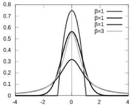
Fig.1. Generalized Gaussian pdf’s for different values of shape parameter в .

class

representing by the feature vectors of the image and the D-dimensional generalized Gaussian distribution is of the form[16].

The mean value of the generalized Gaussian distribution is

П xij Mij |₽1      _ i          7 I Ia

=-----------------j xe idx

2Г(1 + -)Аф, a) -7

P                                   (5)

The GGD is symmetric with respect to ц , hence the odd center moments are zero i.e., E|_Xij-ц..|t = о , t = 1,3,5,…. The even center moments can be obtained from absolute center moments and given by

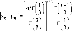
The variance is var(x) = E(x - x)2 = E(x - ц)2 = a2

The model can have one covariance matrix for a generalized Gaussian density of the class. The covariance matrix E can be full or diagonal. In this paper, the diagonal covariance matrix ix considered. This choice based on the initial experimental results. Therefore,

L i=

~ 2

.   ^a iD J

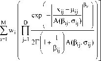
As a result of diagonal covariance matrix for the feature vector, the features are independent and the probability density function of the feature vector is gi(Xr/ 9) = n j=1

xij цу exp------—

|    ^{A( e} ij , a ij )

2Г|1 + Г IA(P ij >a ij ) к     ^{e ij} )

these, the 2D discrete cosine transformation is robust and simple for extracting the features. No serious attempt is made to utilise DCT coefficients for extracting the feature of the texture of the image even though the DCT coefficients are capable of maintaining regularity, complexity of the texture. This is possible since the DCT uses orthogonal transformation of the cosine function. The advantage is DCT can convert the texture of the image from time domain to frequency domain [19]. This motivated us to consider DCT coefficients for extracting the feature vector associated with texture of the image. To compute the feature vector associated with image texture, we divide whole image into M x M blocks. Following the heuristic arguments given by Gonzalez [20], 2D DCT coefficients in each block are computed. These coefficients are selected in a zigzag pattern up to number of 16 coefficients in each block. The 16 coefficients are considered since in many of the face recognition algorithms, it is established that 16 coefficients provide sufficient information in the block. These 16 coefficients in each block are considered as a sample feature vector and the total N=M x M blocks provide Nx16 data matrix for the feature vector of the whole image.

M

p ^(Xr / ^{0 )} = L w i g i ( ^Xr , ⁹ ) i = 1

where, g_{ ( X_r 9 ) is given in the above equation (9).

The likelihood function is

M

D

= П f ij (x rij )

^j =                           (10)

One of the important step in segmentation of texture of an image is extracting the features associated with the texture regions of the image. Texture is the inherent pattern perceived by the image in forming the pixel intensities. Much work had been reported in literature regarding feature vector extraction of texture images [17, 18].Some of the important methods associated with feature vector extraction are PCA, KLT, Fourier transformations and DCT cosine transformations. Among

T

L(9) =П r=1

L w i g i ( ^xr , ⁹) i = 1

T

=n r=1

This implies,

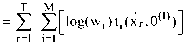
T logL(0) = log П r=1

M

L w i g i ^(x r , ^{0 )} . i=1

Distribution integrated with Hierarchical Clustering

T

=2 log r=1

M

2 w i

exp

D

n

—

A( P ij , ^ ij )

2 Г| 1 + -I A( ₽ j , c j

V ^e ij )

T MD

2 22 log

-I

+

I Pi.

| A( P ij , C y ) t i (X r , 0 ^(l))

To find the refined estimates of parameters W i , ^ ij and c , for i=1,2,3,...M ; j=1,2,,D.

we maximize the expected value likelihood or log likelihood function. The shape parameter pj is estimated using the procedure given by Shaoquan YU (2012) [22].

To estimate w^ ц^and c , we use the EM algorithm which consists of two steps namely, Expectation (E) Step and Maximization (M) Step. The first step of EM algorithm is to estimate initial parameters w^ , ц^ and Cy from a given texture image data.

E-Step:

Given the estimates, 0 ^(l) = ( ц (Р , _с⁽Р ) for i=1,2,...M;

j=1,2,3,…..D

One can estimate probability density function as

M

P ^(Xt / 6 ) = 2 w i g i ( x r , ⁰)

i=1

M-Step:

To maximize Q( 0 , 0 ^(l) ) , we can maximize the term containing w i and containing 0^(l) independently, since they are not related.

To update the component weights w i of the model, we maximize the likelihood function such that ^M

2 w i =1

i = 1

We construct the first order Lagrange type function as

T — T M               _m    f M (l)

22 logtwDt i tx r , ^{0 (l)) +} Y 2 w i ^{— 1}

r=1 i=1                                V i=1

where, у is Lagrange multiplier and maximizing this Lagrange function with respect to w i , we have to differentiate L with respect to w i and equate to zero i.e., —— [L] = 0 implies d w i

The conditional probability of any observation xr belongs to Mth class is

a t m         _        a f m

—22 ^lo g ^(wi^)ti^(xr^{, 0 (l)}) +— y| 2 ^{d w}ir = 1i = 1                       5w i V i = 1

(l) w_i

— 1 I = 0

This implies,

t i (X r / 0 ^(l)) = p((i/x), 0 ^(l)) w i g_i(x r , e ( ^l ) ) p i ⁽x r , ^{0 (l))}

₌ _^wj g j C^x r ,o (^l))_ M

2 w i g i ( x r , ⁰ )

i=1                            (13)

The expected value of L ( 0 ) is

T

2 — t i (x r , 0 ^(l)) -Y = 0

wi

Therefore,

T

2 [ t i^(xr , ^{0 (l)}) ]=Y w i

Summing i=1, 2, 3,…M, we have

Q( ^{0 , 0 (O)} ) = E₆ (l) { logL(0/X r ) }

Following heuristic arguments of Jeff A Bilmes (1997) [23], we get

MT

22[ti(xr, 0,n) ]=Y i=1 r=1

Therefore,

TM

T

2 [ t i^(xr , ^{0 (l)}) ]= Tw i

MD

22 log i = 1 j = 1

+

t i (X r , 0 ^(l) )

Hence, updated equations for w i is

T w ( ^{l + 1)} = 12 i

w ^(l) .g i (x r , 0 ^(l) )

r = 1 Kw^iO x r , 0 ^(l) )

Distribution integrated with Hierarchical Clustering where

^)          )

are the estimates at ith iteration.

This is a non trivial equation, explicit expression for цу is complicated.

Updating цj ?

For updating ц^•, we consider derivative of Q( 0 , 0 ^(l)) with respect to цу for i=1,2,.....M, j=1,2,..D and equate to zero.

—— Q( 0 , 0 ^(l)) = 0 implies ацу

/  L j^log(W i )t , (X r , 0 ^(l)) + L M g^ r , ^t^ r , P® )   | = 0

^дц ij ( r = 1 1 = 1                             r = 1 1 = 1                               J

This implies,

To update ц у , solve equation (21) by using Newton’s Raphson method and obtain ц ^{(1 + 1)} .

This ц(1+1) provides the refined estimates for цу. For explicit estimate of цу, consider the special cases. Case 1: The Gaussian case, Py =2 leads

]T t i (X r , 0 ^(l) ).(x_ri j -ц (^> ) = ]T t i (X r , 0 ^(l) ).(x_ri j -цУ^{+ 1)} ) r=1                                   r=1

This implies, T

L (xrij)w(l)gi(xr,0(l)) u (l+1) = 1=1__________1_______________ ц1|          T

L w ^(l) g i⁽ x r , ^{0 (l) )}

r=1    1

d

Mj

LL log(W i )t i (X r , 0 ^(l)) + IZZ log

t i (X r , 0 ^(l))

= 0

Case 2: consider for Py ^ 1

2 Г1 1 + -| Афу, n j

Since цij involves only one element of feature vector, mean цj, the equation reduces to

M I       IM            I

—LL I - ^log2 r| 1 +|- logA( P ij , a j ) f , (x r . 0 ^(l)) -

⁵№jr = 11 = 1 1        ( P ij J               J

This implies

T

- LL

. t d

x rij    ^ц ij

'^r=1 Sц ij ^A( P ij , ^a ij )

On simplification, we get

^x r1j ^Ц ij

A( P ij , a j )

t i (X r , 0 ^bi = 0

t i (X r , 0 ^(l) ) = 0

T          Г      _     n^ ij ¹

L P ij sign д /il  ^j      t i ^{(X r} , ^{0 )}(^X rij ^-Ц ij ) ^{Э ij -} 1 = ⁰

r = 1          L ^A( P ij , ^a ij ) J

This implies

T

L ti(xr,0(l)) sign r=1

x rij    ^ц у

A( P ij , a ij )

" P ij -1

. ^(x rij ^-M^{) P 1j - 1} = ^{0 for} P ij * ¹

; = ;M^xr_J'« ⁾_S«.

A( P ij , ^a ij )

This implies,

I P g -¹                     _T

_|J     I . ^{) j1} = L t i ( ^xr , O '^sign

И (^{l + 1)} = ^цу

'                   "I P ij "¹

^xrij    P ij

A(₽M j

T

I l (xtiMMx r , ^{0 (i)} ) |^{P ij}

V r=1 J

T

L w ( ^l) g i (x r , 0 ^(l) ) |^{P 1j}

I, и (1 + ¹)!¹

()

For general case: we can also develop a general approximation without using numerical method for updating u(1+1) by adopting an axiom that of the form ц ц ij                                                                                                 ij which must be a weighted average of data vectors with weights provided by some power of the assignment probabilities of those data vectors, notified in part by symmetry of system, and in part by pragmatism leads to

T

L t i (x r , 0 ^(l))^{A(N, P 1}j ⁾(x_tij)

., (l + 1) ₌ 1=1__________________________________ ^ц 1|          t

L t i r , 0 ^(l))^{A(N, e} ij ⁾

r = 1

Therefore,

T Г - 1         T г - 1

о(l)\   •         x rij    ^ЦИ          (          (l)^ Pij^{- 1}                           • x rij    ^ЦУ          (          (1 + 1) \ Pij^{- 1}

L t i ⁽x r , ^{0   )s}ign---------- I x rij -ц ) ^j = L tM, ^{0   )s}ign---------- I x rij ^-ц ) ^j

,                              A(B..,a.•)               j ij /              ,                              A(B..,a..)          \ j ij / r=1                      L v^ij, ij7 _l                               r=1                      L v^ij, i/J where, a(n, Py) is some function =1 for p = 2 and must be equal to 1 for p.. ^ 1, in the case of N=2, we have P1j^1         1J also observed that a(N, p ) must be increasing function ofpy.

Updating q- :

For updating _Q., we consider maximization of q( ₆ , _e (i) ) with respect to a- for i=1,2,.....M, j=1,2,..D. That is

^d Q( 6 , 6 ^(l) ) = 0 implies ^dQ ij

a ( t m           .    , T m                     ^      (25)

— I 22 l°g(w i )t i (x r ,6^(l)) + 22 g i (x r ,6^(l))t i (x r ,6^(l)) I=0

^dQ ij ( r = 1 i = 1                         r = 1 i = 1                            J

Therefore,

d

Sa i,

22 log(W i )t i (X r , 6^(l))+ 221 log

t i (X r , 6^(l))

=0

2Г1 1 + -I A(P ij , Q ij )

Since Q^ involves only one element feature vector, we

have

T

2 t i ^(x r , ^{6 (l)})

d .

— log ^Q ij ^dQ ij

This implies

2^ , 6 ^(l))

r = 1

V^ ij J Ixrij    ^ЦУ l^ij       1

- - - -

This implies

T

2 t i⁽ x r , ^{6 (l)} )

2г| —

Therefore,

ij

Г (l + 1) = ij

The efficiency of the EM algorithm in estimating the parameters is heavily dependent on the number of groups and the initial estimates of the model parameters w_x ^ and Q. for i=1,2,3,.M; j=1,2,..,D.Usually in EM algorithm, the mixing parameter _w and the distribution parameters ц- and _Qy are given with some initial values.

A commonly used method in initialization is by drawing a random sample from the entire data. To utilize the EM-algorithm, we have to initialize the parameters which are usually considered as known apriori. The initial value of w can be taken as w =1/M, where M is the number of texture image regions obtained from the Hierarchical clustering algorithm. Then obtain the initial estimates of the parameters through sample moments as wi= 1/M

Cij= S.D of Mth Class

₌₁ T

^{Ц ij}y 2 x rij

T r = 1

Substituting these values as the initial estimates, the refined estimates of the parameters can be obtained using EM Algorithm by simultaneously solving the equations 19, 24 and 26 using MATLAB.

Once the texture is considered, the main purpose is to identify the regions of interest. The following algorithm can be adopted for texture segmentation using multivariate generalized Gaussian mixture model.

Step 1: Obtain the feature vectors from the texture image using technique presented in feature vector extraction section.

Step 2: Divide the samples into M groups by Hierarchical clustering Algorithm.

Step 3: Find the mean vector, variance vector, ^ ij and Q ij for each class of the multivariate data.

Step 4: Take w i = 1/M, for i=1,2,3,…..M.

Step 5: Obtain the refined estimates of w i , ц- and a^ for each class using the updated equations of the EM algorithm.

Step 6: Assign each feature vector into the corresponding j^th region (segment) according to the maximum likelihood of the j^th component L j .

That is, Feature vector x t is assigned to the j^th region for which L is maximum, where,

— exp

—

A ( P ij , ^ ij )

Lj = max <

П j=1

^{2 r}l ¹ + Tri A ( в , ^" j )

V      ' У )

• VII.    Performance Evaluation

To demonstrate the ability of the developed model, texture segmentation is to be performed by using the dataset of textures available in the Brodatz Texture databases. For each texture image, hierarchical algorithm is employed over the multivariate data of feature vectors to divide in to M groups. For each group, the initial estimate of the parameters w i , ц- and o^ are obtained using heuristics clustering and moment estimators. Using these initial estimates, the refined estimates are calculated based on the updated equations obtained through EM Algorithm. With these values, texture segmentation is performed based of the assignment of the data to a particular group for the likelihood is maximum. Then the segmentation image is drawn based on the application of the developed algorithm. The performance evaluation parameters are calculated and compared with the earlier models.

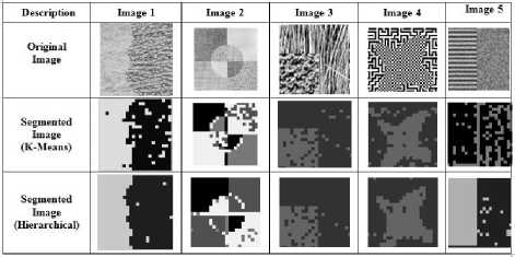
Fig.2. Original and segmented texture images using proposed model with K-means and Hierarchical clustering algorithm.

The performance of the developed texture image segmentation method is studied by obtaining the image segmentation performance measures namely; Probabilistic Rand Index (PRI), the Variation of Information (VOI) and Global Consistency Error (GCE). The Rand index given by Unnikrishnan et al., (2007) counts the fraction of pairs of pixels whose labeling are consistent between the computed segmentation and the ground truth. This quantitative measure is easily extended to the Probabilistic Rand index (PRI) given by Unnikrishnan et al., (2007) [24].

The variation of information (VOI) metric given by Meila (2007) is based on relationship between a point and its cluster. It uses mutual information metric and entropy to approximate the distance between two clustering’s across the lattice of possible clustering’s. It measures the amount of information that is lost or gained in changing from one clustering to another [25].The Global Consistency Error (GCE) given by Martin D. et al., (2001) measures the extent to which one segmentation map can be viewed as a refinement of segmentation.

For a perfect match, every region in one of the segmentations must be identical to, or a refinement (i.e., a subset) of, a region in the other segmentation [26].

The image Performance measures namely, PRI, GCE, VOI are computed for all the five images with respect to the developed model, Generalized Gaussian Mixture Model Hierarchical algorithm to that of other models based on Gaussian mixture are presented in Table 1.

The results show that the segmentation performance measures of the proposed segmentation algorithm based on multivariate generalized Gaussian mixture model are close to the optimal values of PRI, GCE and VOI.

Table 1. Segmentation Performance Measures of the Textured Images

Segmentation Performance Measures

Description	Model	PRI	GCE	VOI
Image 1	GMM-K	0.389	0.351	1.192
	GMM-H	0.428	0.311	1.181
	MGGMM-K	0.511	0.292	1.176
	MGGMM-H	0.732	0.222	1.060
Image 2	GMM-K	0.542	0.580	2.558
	GMM-H	0.558	0.565	2.480
	MGGMM-K	0.648	0.489	2.420
	MGGMM-H	0.721	0.380	1.923
Image 3	GMM-K	0.654	0.325	1.458
	GMM-H	0.685	0.321	1.355
	MGGMM-K	0.780	0.229	1.345
	MGGMM-H	0.848	0.152	1.242
Image 4	GMM-K	0.547	0.351	1.321
	GMM-H	0.558	0.345	1.315
	MGGMM-K	0.633	0.301	1.290
	MGGMM-H	0.721	0.249	1.230
Image 5	GMM-K	0.532	0.590	1.478
	GMM-H	0.569	0.575	1.425
	MGGMM-K	0.558	0.572	1.468
	MGGMM-H	0.625	0.552	1.301

• VIII.    Comparative Study

The developed algorithm performance is evaluated by comparing the algorithm with the Gaussian mixture model with K-means and Hierarchical clustering. Table 2 presents the miss classification rate of the pixels of the sample using the proposed model and Gaussian mixture model.

Table 2. Miss classification Rate of the Classifier

Model	Miss-classification Rate
GMM-K	20%
GMM-H	18%
MGGMM-K	15%
MGGMM-H	12%

From the Table 2, it is observed that the misclassification rate of the classifier with the multivariate generalized Gaussian mixture model is less when compared to that of GMM.

The accuracy of the classifier is also studied for the sample images by using confusion matrix for segmented regions and computing the metrics [27]. Table 3 shows the values of Accuracy, Sensitivity, Specificity, Precision, image texture. Recall, F-Measure for the segmented regions in the

Table 3. Comparative study of MGGMM with Hierarchical clustering Algorithm and earlier Gaussian mixture models.

Description	Model	Accuracy	Sensitivity (TPR)	1-Specificity (FPR)	Precision	Recall	F-Measure
Image 1	GMM-K	0.71	0.72	0.32	0.68	0.72	0.70
	GMM-H	0.73	0.74	0.28	0.7	0.74	0.72
	MGGM M-K	0.75	0.75	0.21	0.72	0.75	0.73
	MGGM M-H	0.81	0.81	0.16	0.85	0.81	0.83
Image 2	GMM-K	0.62	0.69	0.28	0.68	0.69	0.68
	GMM-H	0.64	0.71	0.22	0.72	0.71	0.71
	MGGM M-K	0.69	0.73	0.19	0.76	0.73	0.74
	MGGM M-H	0.74	0.81	0.15	0.82	0.81	0.81
Image 3	GMM-K	0.79	0.72	0.34	0.69	0.72	0.70
	GMM-H	0.82	0.74	0.31	0.72	0.74	0.73
	MGGM M-K	0.86	0.79	0.26	0.75	0.79	0.77
	MGGM M-H	0.89	0.84	0.21	0.89	0.84	0.86
Image 4	GMM-K	0.81	0.71	0.33	0.65	0.71	0.68
	GMM-H	0.82	0.72	0.29	0.68	0.72	0.70
	MGGM M-K	0.84	0.76	0.27	0.72	0.76	0.74
	MGGM M-H	0.86	0.82	0.24	0.81	0.82	0.81
Image 5	GMM-K	0.58	0.68	0.38	0.59	0.68	0.68
	GMM-H	0.65	0.72	0.32	0.62	0.72	0.72
	MGGM M-K	0.62	0.70	0.34	0.61	0.70	0.71
	MGGM M-H	0.69	0.78	0.20	0.72	0.78	0.74

From Table 3, it is observed that the F-measure value for the proposed classifier is more than the earlier Gaussian mixture models. This indicates that the proposed classifier perform well than that of Gaussian mixture model.

• IX.    Conclusions

This paper addresses a new and novel method for segmenting the texture of an image using multivariate generalized Gaussian mixture model distribution. Here, the feature vector representing the texture of the image is derived through DCT coefficients. The texture of the whole image is characterized by a multivariate generalized Gaussian mixture distribution. The generalized Gaussian distribution includes Gaussian and Laplace distributions as particular cases and several other probability models which are platy-kurtic, lepto-kurtic and meso-kurtic. Hence, this method is capable of characterizing the textures of several images for which the feature vector may be one among having platy-kurtic, lepto-kurtic and meso-kurtic distributions in the image regions. The model parameters such as shape and scale are estimated through EM algorithm. The shape parameter is estimated using sample kurtosis for reducing the computational complexity with respect to convergence of EM algorithm. The initial values of the model parameters are obtained by integrating hierarchical clustering with the moment method of estimation. Experimentation with five randomly taken images from Brodatz texture database supported the superior performance of the proposed algorithm over the texture segmentation algorithm based on Gaussian mixture model with respect to the segmentation performance measures such as PRI, GCE and VOI. The confusion matrix computed along with F-measure also supported the outperformance of the proposed algorithm. The texture segmentation algorithm is useful for analyzing several image textures for efficient analysis of the systems. It is possible to further extend this proposed algorithm by considering other methods of initialization of parameters such as fuzzy c means, MDL and MML. It is also possible to induce neighborhood information in extracting the feature vector which will be considered elsewhere.