Study on Diesel Engine Fault Diagnosis Method based on Integration Super Parent One Dependence Estimator

Published Online February 2011 in MECS

Diesel engine is a complex machine and a multi-interference system. The relationship between its input and output variables, fault and sign is unobvious and uncertainty. Poor working conditions easily lead to signal distortion etc. These have greatly increased the types of diesel engine fault diagnosis difficulty. In recent years, scholars from various countries for the diesel engine fault diagnosis methods have made a lot of related.

Bayesian diagnosis is established based on the probability density function. Compared to the diagnosis based on the failure mechanism, it has smaller diagnostic error rates. So it has an extensive application. With the development of information and automation technology, a lot of running data and diagnostic data has been accumulated and it is possible to calculate the prior probabilities of Bayesian method. However, in many practical fields, the independency assumption of Naïve Bayes (NB) does not hold. Therefore, many researches are mainly about how to use some technology to find a most favorable topology among all possible network structures. At present, such technologies can be summarized into two categories: heuristic search and correlation analysis. To relax the independency assumption, the researchers have done a lot of work. With the development of modern science technology and the degree of automation, diesel engine fault diagnostic technique has undergone significant changes and Bayesian diagnosis become one of the most efficient diagnosis methods.

Among all these improving approaches, One-Dependence Estimators (ODEs) [1] are simple but effective classifiers. ODEs are very similar to NB but they also allow every attribute to depend on, at most, another attribute besides the class. Both theoretical analysis and empirical evidence have shown that ODEs can improve upon NB’s accuracy when its attribute independence assumption is violated. Tree Augmented Bayesian Network (TAN) [2] is kind of ODE which provides a powerful alternative to NB. Super Parent-One-Dependence Estimators (SPODEs) [3] can be considered a subcategory of ODEs where all attributes depend on the same attribute. L.X. Jiang [4] et al adds the parent node for some attributes in Bayesian network using conditional mutual information. Aggregating One-Dependence Estimators (AODE) ensembles all SPODEs that satisfy a minimum support constraint [5] and estimate class conditional probabilities by averaging across them. This ensemble has demonstrated very high prediction accuracy with modest computational requirements. However, it is based on an implicit assumption that all SPODEs have the same or equivalent learning ability. But the leaning ability of different Bayesian networks is different. Simply averaging all SPODEs may scale up the influence of the bad performance classifiers so as to affect the final classification result. WAODE [6] is an improvement of AODE. It uses conditional mutual information to determine the weight of each SPODE. HNB [7] and HODE [8] are another two improved versions of AODE. Addressing how to select SPODEs for ensemble so as to minimize classification error, Yang Y et al [9] proposed five selection methods, minimum description length (MDL), minimum message length (MML), and leave one out (LOO), Backward Sequential Elimination (BSE) and Forward Sequential Addition (FSA). Their experimental results showed that measuring ensembles outperforms measuring single SPODE and model selection for SPODE is advisable since the selection makes differences. In addition, Li Nan et al [10] take each SPODE as a production model and weight each SPODE using the fitting degree of the model to data.

• II.    SuperParent-One-Dependence Estimators

(SPODE S )

Assume D is a set of training instances,

A = { A  A }

• ^{1    , n} is the attributes variable set, where N is the number of attributes, ^C is a class variable, ^c is a value of C. ^{a 1 , L , ai , L , an} are the attribute value of

for which the base probability estimates are inaccurate, ensemble of all SPODEs except for those who have less than 30 training instances. Hence, AODE classifies an instance ^X by using the following equality.

P ( c\X ) =

^ ⁿ ^

X , :1 ₅ , ₅ n л F ( a , ) _й m^{P (} c , ^ ^П ^{P (} a j ¹ c , a - )

j = 1

\1 <  i <  n л F ( a , ) >  m \ x P ( X )

Where F ( a ⁱ ) is a count of the number of training examples having attribute-value a ⁱ and is used to enforce the limit m that we place on the support needed in order to accept a conditional probability estimate. In the presence of estimation error, if the inaccuracies of the estimates are unbiased the mean can be expected to factor out that error.

• III.   New Approach to weight SPODE

A data sample of n attributes can potentially have n SPODEs, each alternatively taking a different attributes as the super parent, as shown in Fig.1. In this paper, we consider the diversity of SPODE and its corresponding NB and propose a new approach to weight SPODE.

A L A L A

^{1 ,, i ,, n} respectively.

A SPODE requires all attributes to depend on the same attribute, namely the super parent, in addition to

the class. Let

SPODEA

denote the SPODE with

SPODE super parent At.            ^At

will estimate the

probability of each class label ^c given an instance ^X as follows:

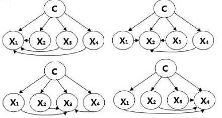
Fig.1. 4 SPODEs with 4 attributes

P ( c I X ) =

P ( c , X ) P ( X )

P ( c , a. ) П P ( a j I c , a , ) _____________ j = i,j * , ____________________

P ( X )

Since the above equality holds for every SPODE, it also holds for the mean over any subset. An ensemble of k SPODEs corresponding to the super-parents A 1, … , A k estimates the class probability by averaging their results as follows.

P ( c I X ) =

k

X ^P ( ^c , a ) П ^P ( a j ^{1 c} , a )

i=1                j * i k x P (X)

A. Diversity of SPODE and its corresponding NB

A natural question is that how well a SPODE can perform in predictive tests. If the prediction result for a test instance by using a SPODE is same with that by using NB, we can say that the performance of the SPODE is not very well. We would rather use its corresponding NB than the SPODE since the structure of SPODE is more complex than simple NB and the parameter estimation needs more time while the performance are the same.

Definition 1 If a test instance ^X is classified

AODE selects a limited class of 1-dependence classifiers and aggregate the predictions of all qualified classifiers within this class. To avoid including models

to the same class by using SPODE and by using NB, then we say the performance of SPODE and NB is equivalence.

Definition 2 Suppose there are m classes. Let Diver ( SPODEA, , nb) be a m ^x m square array such

_that Diver ij

is the number of test examples assigned

to class

SPODE ^{c i} by             ^At

c with and to class j

by its

corresponding NB. Let ^{| Diver |} be the number of all

test examples. The diversity of

SPODEA

and its

corresponding NB is defined as follows.

Diff ( A t ) = La ^{1 -} p

Where a be the probability that the and its corresponding NB perform the same,

(4) SPODE_A ^в be the

probability that the

SPODEA

and its corresponding

NB agree by chance. They are respectively defined as follows.

m

E Diver , a = ij¹-----

| Diver |

tot =

f- (1d« ( A ) * 0)

E Diff ( A ) ‘ ='

i = 1

Where ^{Diff ( A} t ⁾

Since (1) holds

n

E tot ='

is defined in (4) and t =        .

for every SPODE, we can

estimate the probability of each class label ^c given an instance ^X as follows:

nn

E ® t^{p (} c ^, a t ) П P ⁽ a , \ c ^, a t ) t = 1 . j = 1, j * t

P ( c\X ) H

P ( X )

P ( c ) fl P ( a,\c )

n

, E ^to t * 0

t = 1

■ j =1 __________ P ( X )

, else

mm e=E (E i=1 j=1

e ^0^, ) | Diver | “Ji Diver |

The proposed classifier is named WSPODE.

WSPODE classifies a newly instance using (9) as well.

Further, we have the following discussion.

When Diff(At) =0, we can get α =1. It means that the classification results using

SPODEA

and its

corresponding NB are completely same. The two classifiers agree on every example.

When Diff (At)=1, we can get α=β. It means that

SPODEA

and its corresponding NB equals that expected by chance.

When iff ( ^t )>1, we can get α < β . It means that agreement is weaker than expected by chance. In another words, the chance of the two classifiers obtain the same classification is slim.

If the diversity between the augmented naïve bayes and the simple naïve bayes is small, it has no need to expand the network structure of NB. Because of the complexity of probability estimation is closely related to the network structure.

From the above discussion, we can get the conclusion that the diversity between the augmented SPODE naïve bays         At and the simple naïve bays increases with the increase of the value of Diff(At).

Diff ( A )

Therefore, we take t as the weight of SPODEA argmaxP(c| X) c

The value of ^wt can determine the number of SPODEs used as well as the importance of every SPODE. For example, if      w t = ⁰

, w , * 0( j e [1, n ], j * t )                         .      . .

and j                    , we actually only select n -1     SPODEs. In a extreme case

n

E Diff ( A ) = 0

when i-1             , we will use NB to classify all test samples. But this kind of situation is rare. Because it means that all SPODE perform exactly the same with NB. Every SPODE and its corresponding NB agree on every example.

• IV.    Algorithm description

In this section, we describe our algorithm for training and inference. During the training phase, the goal is to determine the weight of every SPODE using (7). The learning algorithm for WSPODE is depicted as follows. In classification phase, use (8) to classify a newly instance without class label.

• B. SPODEs Ensemble

According to the above discussion, firstly we give

SPODEA

the definition of the weight of

Definition 3 Let ® t represents the weight of

SPODEA

w t is defines as:

Algorithm. WSPODE (D)

Training phase:

Input: a set D of training examples

Output: a Improved Naive Bayesian Classifier for D

Using NB to classify training examples in D and store the result;

For each attribute At (t =1,^ , n)

There is a Diver[m][m], where m is the number of class labels;

For each example l in D delete its class label

If l is classified to ^{c j} by

SPODE        c

^At and to ^k by NB (j, k =0,…,m-1)

Then Diver[j][k]= Diver[j][k]+1;

For j=0 to m-1, k=0 to m-1

Diver[j][k]= Diver[j][k]/the size of D;

Compute α using (5);

Compute β using (6);

Compute Diff(At) using (4);

Compute ® t using (7);

Sum=0;

For i=1 to n sum=sum+ ® i ;

For i=1 to n ® ‘ = ® ‘ /sum;

Classification phase:

Input: the Improved Classifier built in training phase, a newly instance X

Output: the class label c of X

For i=1 to m

Compute P(ci|X) using (8), the parameters are obtained in training phase;

arg max P ( c_i | X )

c=       ^{c i}              .

• V.    Experiments

• A.    Experimental settings

• (1)    Test data

In this paper, we choose 16 UCI datasets (shown in table II ) and 3 foul diagnostic datasets of diesel engine (shown in table Ш ). WD615 diesel engine valve fault diagnosis data is used to de simulation experimental.

The datasets of diesel engine is got by The Dewetron Combustion Analyzer as fig2-5. The Dewetron Combustion Analyzer systems are used for engine research, development and optimization. Also for component development and testing, such as ignition systems, exhaust systems and valve control gear. Through measuring diesel engine cylinder pressure and crank angle, eigenvalues are calculated to analysis.

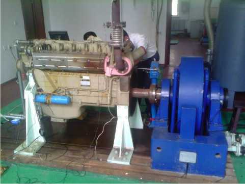
Figure.2. WD615 diesel engine

Assume that the number of training instances and attributes are s and n respectively. The number of classes is m. The average number of values for an attributes is v.

In order to train the weight of every SPODE, we

SPODE            SPODE compute Diver (        At , NB) for each At using the training data without the class label. Hence, compared to AODE, it needs more o(smn) time complexity.

In classification phase, the time complexity of the WSPODE is o(mn2). It is just the same as AODE.

TableI. Time Complexity algorithm      Training      classification

_AODE       o ( mn ²) o ( mn ²)

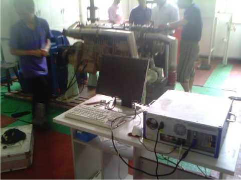
Fig.3. Dewetron Combustion Analyzer

WAODE     o ⁽ sn 2 ^{+ n} )       o ⁽ mn 2 )

LODE      o ( sn 2 + sn )       o ( mn 2 )

WSPODE o ( sn 2 + smn )     o ( mn 2 )

TableIII. Diesel datasets

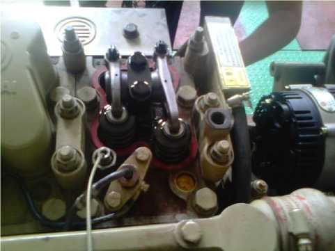
Fig.4. P ressure S ensor

	number	Description
size	1600	When the load is 0Nm, 100 Nm, 200 Nm, 300 Nm and 400 Nm, collect 2000 cycles’ data respectively. The datasets are denoted as Diesel1,
.A#	12	Diesel2, Diesel3, Diesel4 and Diesel5. Each dataset has 2000 records. © speed; © maximum Cylinder Pressure; © phase of maximum Cylinder Pressure; © phase of maximum of rising rate of maximum Cylinder Pressure; © phase when energy conversion reaches 50%; © phase of starting burning,; © phase of
C#	4	ending burning; © phase difference between burning start and burning end; ® mean indicating effective pressure; © net mean effective pressure; © indicated power © Both intake valve clearance and Exhaust valve clearance are small; © Intake valve clearance is too small; © Both intake valve clearance and Exhaust valve clearance are too large; © normal clearance.

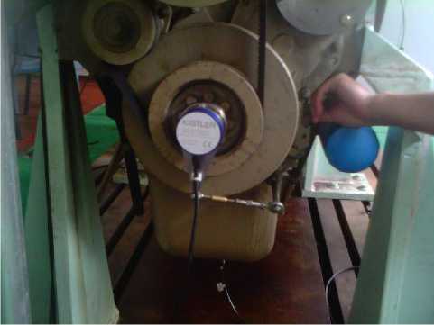
Fig.5. C rank A ngle S ensor

All datasets are preprocessed with the help of WEKA1 software before using. Use the supervised filter Discretize in WEKA to discretize all the numeric attributes; Use the unsupervised filter Remove in WEKA to remove useless attributes. The discretized data is showed in table © .

TableII. UCI datasets

I d	dataset	size	C #	A #	Id	dataset	size	C #	A #
1	breast_ w	699	2	9	9	machine	209	7	7
2	car	172 8	4	6	1 0	promoter	106	2	57
3	diabete s	768	2	6	1 1	sonar	208	2	21
4	Flags	194	6	30	1 2	tic_tac_t oe	958	2	9
5	flare	138 9	2	13	1 3	vote	435	2	16
6	heart_h	294	5	9	1 4	vowel	990	1 1	14
7	iris	150	3	4	1 5	wavefor m	500 0	3	19
8	lymph	148	4	18	1 6	zoo	101	7	16

1

• (2)    Validation method

• 10 runs of 10-folds CV test for comparing the classifier performances. Each datasets are divided into 10 almost equal-sized blocks randomly, and in each validation, one block was used for test data and the remaining blocks were used for training classifiers. Average all 10 runs as the final results like table V .

• (3)    Measurement

Throughout all the tests, we measured the classification error rate, i.e., the percentage of incorrectly classified instances.

TableIV. partial result of mixed conditions discretization

nn	max1	amax1	adpmax	class
(1796.37-1799.17]	(76.30-76.98]	(5.95-6.45]	(6.05-6.25]	B
(1796.37-1799.17]	(75.37-76.30]	(6.45-6.75]	(7.45-inf)	B
(1796.37-1799.17]	(76.30-76.98]	(4.65-5.25]	(6.05-6.25]	B
(1796.37-1799.17]	(76.98-77.45]	(4.65-5.25]	(6.25-6.55]	B
(1782.78-1791.25]	(78.29-inf)	(5.95-6.45]	(5.55-5.75]	A
(1782.78-1791.25]	(77.45-78.29]	(6.75-7.15]	(5.75-6.05]	A
(1782.78-1791.25]	(77.45-78.29]	(4.65-5.25]	(5.55-5.75]	A
(1782.78-1791.25]	(76.98-77.45]	(4.65-5.25]	(3.55-5.05]	A
(1782.78-1791.25]	(77.45-78.29]	(5.25-5.95]	(5.05-5.55]	A
(1791.25-1796.37]	(77.45-78.29]	(6.45-6.75]	(5.75-6.05]	A
(1796.37-1799.17]	(75.37-76.30]	(5.25-5.95]	(6.55-7.45]	C
(1796.37-1799.17]	(75.37-76.30]	(6.75-7.15]	(7.45-inf)	C
(1796.37-1799.17]	(-inf-75.37]	(7.15-inf)	(6.55-7.45]	C
(1796.37-1799.17]	(75.37-76.30]	(7.15-inf)	(7.45-inf)	C
(1796.37-1799.17]	(76.30-76.98]	(6.75-7.15]	(7.45-inf)	C
(1806.1-1808.80]	(76.30-76.98]	(7.15-inf)	(3.55-5.05]	D
(1806.1-1808.80]	(76.98-77.45]	(7.15-inf)	(6.25-6.55]	D
(1806.1-1808.80]	(-inf-75.37]	(7.15-inf)	(7.45-inf)	D
(1806.1-1808.80]	(76.30-76.98]	(6.75-7.15]	(6.25-6.55]	D

(1806.1-1808.80]	(76.30-76.98]	(7.15-inf)	(7.45-inf)	D
(1806.1-1808.80]	(76.30-76.98]	(5.25-5.95]	(6.55-7.45]	D

Error rate= number of incorrectly classified instances / the total number of instances of prediction. (4) Comparison algorithms

This paper compares the proposed method with AODE , WAODE and LODE in table d .

• B.    Experimental results and Analysis

The experimental results are shown in table 4. Since the average error rates of different classifiers are very close. So we compare each two algorithms A-B via two tailed t-test with a 95 percent confidence level. The results are shown in table 5, where win indicates that algorithm A obtained significantly lower average error rate than algorithm B, draw indicates that A and B haven’t significant differences, and loss indicates that A obtained significantly higher average error rate than algorithm B. From table ^ , we can see that WSPODE outperforms AODE on 9 datasets, outperforms WAODE on 8 datasets, and outperforms LODE on 8 datasets.

TableV. 10 runs error rate of diesel engine data2

dataset	runs	AODE	WAODE	LODE	WSPODE
data2d	1	8.06%	8.12%	7.81%	8.12%
data2d	2	7.62%	7.44%	7.31%	7.81%
data2d	3	7.69%	7.81%	7.56%	7.94%
data2d	4	8.00%	7.75%	7.69%	7.81%
data2d	5	7.56%	7.56%	7.63%	7.75%
data2d	6	7.81%	7.94%	7.50%	7.81%
data2d	7	8.13%	8.00%	7.57%	8.00%
data2d	8	7.75%	7.75%	7.69%	7.82%
data2d	9	7.69%	7.31%	7.37%	7.75%
data2d	10	7.56%	7.63%	7.75%	7.44%
	mean	7.79%	7.73%	7.59%	7.83%

TableVI. detailed results of error rate and standard deviation dataset AODE WAODE LODE WSPODE breast_w 3.02±0.17 2.98±0.11 2.95±0.17 2.92±0.18 car 8.09±0.36 8.92±0.29 8.04±0.35 7.73±0.43 diabetes 21.69±0.28 21.81±0.36 21.60±0.34 21.62±0.37

Flags 39.82±1.20 39.77±1.36 41.04±0.99 39.31±1.24 flare 19.80±0.57 18.20±0.25 19.41±0.68 18.08±0.31 heart_h 14.59±0.38 14.52±0.55 14.55±0.36 14.62±0.37 iris 6.54±0.84 6.88±0.72 6.54±0.84 6.08±0.76 lymph 14.77±0.85 13.41±1.38 14.83±0.97 13.54±1.46 machine 9.48±0.49 9.24±0.50 9.48±0.58 9.43±0.60 promoter 10.93±1.47 10.03±2.13 23.22±2.27 9.77±1.81 sonar 14.22±0.90 13.21±0.78 14.32±0.78 13.84±0.99 tic_tac_toe 25.88±0.39 27.05±0.49 25.73±0.35 25.62±0.36 vote 5.58±0.16 5.70±0.18 5.60±0.16 5.65±0.19

	vowel	13.04±0.5715.94±0.52 10.76±0.61 12.60±0.49
waveform 13.73±0.13 13.64±0.14 15.20±0.40 13.69±0.15
	zoo	5.21±0.91	5.21±0.91	5.21±0.91 5.13±0.90
	Diesel1	17.52±0.22 17.54±0.29 17.11±0.33 17.33±0.30
	Diesel2	14.26±0.29 13.57±0.26 14.09±0.26 13.84±0.31
	Diesel3	18.60±0.29 19.01±0.20 18.32±0.32 18.38±0.17
	Diesel4	17.05±0.26 17.03±0.28 17.22±0.21 16.95±0.26
	Diesel5	8.06±0.15	8.16±0.19	8.13±0.14 7.98±0.12
	mean	14.38±0.5214.37±0.57 14.92±0.57 14.00±0.56
TableVII.		the compared results of two-tailed t-test
id	WSPODE WSPODE WSPODE LODE -AODE -WAODE -LODE -AODE				LODE -WAODE	WAODE -AODE
1	win	draw	draw	win	draw	draw
2	win	win	win	draw	win	loss
3	draw	draw	draw	draw	draw	draw
4	draw	draw	win	loss	loss	draw
5	win	draw	win	draw	loss	win
6	draw	draw	draw	draw	draw	draw
7	draw	win	draw	draw	win	loss
8	win	draw	win	draw	loss	win
9	draw	draw	draw	draw	draw	draw
10	draw	draw	win	loss	loss	draw
11	draw	win	draw	draw	loss	win
12	win	win	draw	win	win	loss
13	draw	draw	draw	draw	draw	draw
14	win	win	win	win	win	loss
15	draw	draw	win	loss	loss	draw
16	draw	draw	draw	draw	draw	draw
17	win	win	loss	win	win	draw
18	win	loss	win	win	loss	win
19	win	win	draw	win	win	loss
20	win	draw	win	loss	loss	draw
21	draw	win	win	draw	draw	draw
total	10\11\0	8\12\1	10\10\1	6\11\4	6\7\8	4\12\5

• VI.    Conclusions

In order to improve artificial intelligence diesel engine diagnosis accuracy. This paper relaxed the assumption so as to gain smaller classification error rate, took the study of one-dependence estimator, and proposed a new strategy. It took advantage of the diversity and its corresponding NB to weight the SPODEs. Through the comparison experiments with the existing AODE, WAODE and LODE by University of California Irvine (UCI) and 5 diesel engine datasets collected by our lab, the results verified the effectiveness of the proposed algorithm.