Sufficient relative minimum conditions for discrete-continuous control systems

Hybrid systems, which include systems with variable structure [1] , discrete-continuous [2] , logic-dynamic [3 , 4] , impulsive [5] , and some other systems, firmly took their place in the theory of optimal control. They are also sometimes referred to as “heterogeneous”. A considerable part of scientific conferences and journals are devoted to that field. They propose corresponding mathematical models and methods of investigation for each type of such systems.

We consider a class of optimal control problems, which is characterized by the change of descriptions with time in terms of controlled differential systems. For this class, a two-level model of a discrete-continuous system (DCS) is proposed in [2 , 6 –8] . Its lower level describes the continuous uniform controllable processes at the individual stages. The upper (discrete) level integrates these descriptions into a unique process and controls the functioning of the entire system as a whole to ensure the minimum of the functional.

(0 Ailamazyan Program Systems Institute of RAS, 2020

Y-4.0

The sufficient optimality conditions for the model were established and control improvement methods were developed [6 –8] . These conditions allow one to find the global minimum of the functional of optimal control problem. However, in practice, the admissible control set may have a complex structure with specific state constraints. Therefore, most of the computational methods suggested in the literature yield to a relative minimum of the functional. However, it is impossible to verify that the suggested solution provides a relative minimum.

The purpose of this work is to fill the gap. Namely, we derive sufficient relative minimum conditions that can be used for the evaluation of the proposed solution and enable one to construct new numerical methods.

• 1.    Model of the discrete-continuous system

We consider the abstract discrete controllable system [9] :

• (1)   x(k + 1) = f (k, x(k), u(k)) , k E K = {k i ,ki + 1,...,k F },

where k is the step (stage) number, time is not necessarily physical, x and u are variables of state and control, respectively, f is an operator. All these ob jects have an arbitrary (possibly, different) nature for different k, U (k, x) is a set given for each k and x, k I , k F are the initial and final steps, respectively. On some subset K ‘ C K , k F / K ‘ , there is a continuous system of the lower level

c

• (2)      x c =       = f c (z,t,x ^c ,u ^c ),      t E T (z) = [t i (z),t F (z)],

x ^c E X c (z,t) C R ^n(k) , u c E U ^c (z,t,x ^c ) C R ^p(k) , z = (k, x, u d ).

Here U ^c (z,t,x^c) is the given set.

The right-hand side operator (1) is given by f (k,x,u) = 9(z,Yc), where

Yc = (ti,xc, tF,xCF) E rc(z), rc(z) = {Yc : ti = т(z), xc = ^(z), (tF,xCf) E FF,(z)} .

Here z = (k,x,u ^d ) is a set of the upper-level variables playing the role of lower-level parameters, u ^d is a control variable of arbitrary nature, t I = т (z), x ^cc = ^(z) are given functions of z.

The solution of this two-level system is the set m = (x(k),u(k)) called the discrete-continuous process . For each k ∈ K ‘ , u(k) = (u ^d (k), m ^c (k)), where m ^c (k) E D ^c (z(k)) is a continuous process (x ^c (k, t),u ^c (k, t)), t E T (z(k)). Here D ^c (z) is the set of admissible processes m ^c , satisfying with the specified differential system (2) with additional restrictions. It is supposed that u ^c (k,t) is piecewise continuous and x ^c (k,t) is piecewise smooth (at each discrete step k). Let us denote the set of elements m satisfying all the above conditions by D and call it a set of admissible discrete-continuous processes.

For the model (1) , (2) , we consider the problem of finding the minimum on D of the functional I = F(x(k _F )) under fixed k I = 0, k F = K , x(k I ) and additional constraints

• (3)    x(k) E X (k), x ^c E X ^c (z,t),

• 2.    Control improvement and optimality sufficient conditions

X (k), X ^c (z, t) are the given sets.

The model (1) , (2) is suitable to describe various nonuniform controllable processes. Its lower level describes the continuous controllable processes at the individual stages. The upper one integrates these descriptions into a unique process. In the problems of optimization, both levels are interacting. Interaction with each subsystem of the lower level is through the boundary of this subsystem and the corresponding continuous process γ ^c .

The sufficient optimality conditions for this model we derive by analogy with Krotov’s sufficient conditions for discrete and continuous systems by eliminating the discrete chain and the differential system from the constraints of the sets D and D ^c , scalar functions (functionals) ф(k,x), ф ^c (z,t,x ^c ) are introduced. The latter is the parametric family (with the parameter z) of the smooth functions, where z = ^k, x(k), u ^d (k)^. The following generalized Lagrangian is constructed:

L = G (x(kp )) —    ^^ R (k,x(k),u(k)) +

K \ K ' \k _F

+ ^(G ^c ( z(k),Y c ( z(k) )) — K ^′

— j^ R ^c (z[k), t, x ^c (k, t), u ^c (k, t)) dt^, T ( z ( k ) )

G(x)

R(k, x, u)

G c (z,Y c )

R ^c (z, t, x c , u c )

M ^c (z,t) l c (z)

^ ^(k)

= F (x) + ф(k F , x) — ф Qu,x(k i )) ,

= Ф ( k + 1,f (k,x,u) ) — ф(k,x),

-

-

Ф^к + 1, 9(z, Y c )) + ф(к, x) + ф ^c (z, t F , x ^c _F ) — ф ^c (z,t I ,x I ),

= ф Х^Т f c (z,t,x ^c ,u ^c ) + ф ^c t (z,t,x^c),

= sup { R ^c (z, t, x c , u c ) : x c € X ^c (z,t), u ^c € U ^c (z, t, x c ) } ,

= inf {Gc(z,Yc) : Yc € F(z), xc € Xc(z,tF)} , sup {R(k,x, u): x € X(k), u € U(k,x)} , t € K \ K', — inf |lc(z) : x € X(k), ud € Ud(k,x)} , к € K', l = inf{G(x) : x € Г П X(K)}.

Here ф Х с is the gradient of ф ^c in the space (x ^c ), T denotes transposition.

Theorem 1. Let there be a sequence of discrete-continuous processes {m _s } ⊂ D and functionals φ, φ ^c such that

• 1)    ^ ^c (z,t) is piecewise continuous for each z;

• 2)    R (_k, x _s (k), u _s (k)) ^ ^(k) , к € K ;

• 3)    / t ( z ) (R c (z s , t, x S (t), u S (t ^c )) — ^ ^c (z _s , t )^ dt ^ 0 , к € K ' and t € T (z S ) ;

• 4)    G ^{c (z} s ^,Y S' ^{) — l} c ^(z s ⁾ ^ ⁰ , ^{k €} K ' ;

• 5)    G (_x_s(tp )) ^ l.

• 3.    Relative minimum

Then the sequence {m _s } is a minimizing sequence for I on D .

The proof is given in [6, 8] .

Suppose that x^c(k,t i ) = £(k,x(k)), k i ,k F ,x(k i ),t i (k),t F (k) are fixed, there are no constraints for state variables of both levels and upper-level control variables, lower-level subsystems do not depend on u d , X ( k ) = R ^d(k) , X ^c ( k , t ) = R ^p(k) , U ( k , x ) = R ^r(k) , and the used constructions of sufficient optimality conditions are such that all the following operations are valid. Let x(k) and x ^c (k,t) be elements of D , and there exists, at least one value u(k) and u ^c (k,t) with corresponding x(k + 1), x ^c (k, t), i.e., u(k), u ^c (k, t) are inner points of U , U ^c .

Let us denote by D ϵ a subset of elements of D that satisfy additional conditions

|x(k) — x(k)| < e,   |x ^c (k,t) — x ^c (k,t)| < e, e> 0.

We will say that on a discrete-continuous process m a relative minimum of I is attained on D if I (m) = inf I.

D ϵ

On the basis of the above-mentioned theorem, the sufficient conditions for the relative minimum of the functions R, R ^c are as follows

• (4)                 dR = 0,                    dP ^c = 0,

• (5)                d ² R < 0,                   d ² P ^c < 0,

where P ^c (k,t,x ^c ) = sup R ^c (k, t, x ^c , u ^c ).

u ^c ∈ U ^c

We can make these conditions more detailed for the problem with a free terminal state, i.e., x(k I ) is fixed and x(k _F ) is free, x(k _F ) E R ^d(k) . In addition, the set r ^c (z) is given by r ^c (z) = {y ^c : x / = ^(z), x F E R ^p(k) }.

It follows from (4) that

• (6)           R x = 0,     R u = 0,      P x c = 0,      P x = 0,

where dR = R T Ax + R T Au. The derivatives are calculated on the element m.

From (6) one has

^(k) = H,    H u = 0,

H(k,^,x,u)= ^ (k + 1)f(k,x,u),     k E K \ K ‘ ,

^ c (M) = -H c ,     )(М) = H.

H(k^x ^ ,x ^cF ) = ^ T (k + 1)9(k,x c , x ^cF ),      k E K ‘ \ k F ,

H ^c (k, t, x, x c , u c ) = ^ ^cT (k, t)f ^c (k, t, x^c, u c ),       H c = sup H c .

u ^c

The condition d2R < 0 or d2R = AxTRXXAx + 2AxTRXuAu + AuTRuuAu < 0

for k ∈ K \ K ^′ , as in [10] , can be replaced by the equivalent conditions

• (9)                        max d?R < 0,

∆ u

Au ^T R uu Au <  0.

Assuming that the maximum is reached in a stationary point, we have R Tu Ax + R _uu Au = 0, from which we get Au = - R —^ R xu Ax. Then max d² R = Ax^T (R _xx - R _Xu R^^RT_u )Ax.

∆ u

Let us take into consideration negative definite matrix G(k); with regard to R _xx , R _xu , R _uu the condition (6) can be rewritten in the form:

• ^{(11)    ст(к)} = f XT ^(k ⁺ 1Yf x ⁺ H xx ^— H xu H—uH ux ^— G^(k), where a(k) = ф _XX (k,x). Let us now consider the following condition d 2 P ^c = Ax ^cT P _X ^c c _x c Ax ^c + 2Ax ^cT P x c x Ax + Ax ^T P xx Ax <  0.

The matrix of second derivatives is:

M =

c xcx

c xx

We introduce the matrix

0 *

/ 0 2    0

0   0 3

,

where matrices 02, 03 are negative definite. Then we can represent the condition d2Pc < 0 in the form M = O*. Hence it follows that

• (1^{2)    j c} = -H X c x c ^- H X c ^ c a^{c -} CT c H X' T ^ c ^- ^ c H c^c ^ c o^c + ^O 2 (k, t),

• (13)     в = -H Xx — ^H , — H x^ c ш - с П . . ш + О з (к, t),

• ⁽¹⁴⁾     Co = —H Xx C ^- H X c ^ c ^{ш -} O^ c x ^- O c H, с ф ^ш.

It is easy to see that on the set K ^′

j(k) = ^ T j(k + 1)^ x + H xx + X x ^ x i j(k + 1)e x +

• (15)              + e x j(k + 1)9 x I X x + X x^ j(k + 1)^ x c X x +

+ X T j ^c (k,t i )X x + X x C T (k,t i ) + c(k,t i ).

Here j ^c (k,t) = ф X c _X c (k,t,x,x ^c ) , e(k,t) = ф X_X (k,t,x,x ^c ) , c(k,t) = = ф Xx C ^(k,t,X,x ^c )•

Consider now first and second-order minimum conditions for G , G ^c . We denote by Γ the subset of elements of the set D such that |x(k _F ) — x(k _F )| < e, e > 0 and by Г ^с the subset of elements of the set D such that |x(k _F ) — x(k _F )| < e, |x ^c (k, t _F ) — x ^c (k, t _F )| < e, e > 0. By virtue of Theorem 1, the sufficient conditions for relative minimum of the functions G, G ^c on the sets Γ , Γ ^c are as follows:

• (16)                dG = 0,                   dG ^c = 0,

d ² G > 0,                  d ² G ^c > 0.

It follows from condition (16) that

G x F = 0,    G x = 0, G x c = 0.

Then

• (17)      ^(k F ) = -F x f ,      <(k,t F ) = - H x cF , X(k,t F ) = 0.

From condition d?G >  0 for k E K \ K ‘ we have j(k _F ) = - F _x F _x F +O 1 , where the matrix O 1 is positive definite.

On the other hand, in analogy with the peceding condition d?Pc < 0, the condition d2Gc > 0 can be represented in the form jc(k,tF) = eTc j(k + 1)0xc + Hxcxc, F    FF

c(k,t _F ) = 0,      e(k,t _F ) = 0.

As before, all the derivatives are evaluated on element m .

Theorem 2. In order for element m to be a relative minimum of I on D , it is sufficient that there exist vector functions ψ, ψ ^c , λ, matrices σ, a c , в, w, and negative definite matrices 0(k) , —© 1 (k) , © ² (k,t) , © 3 (k,t), which satisfy conditions (7) , (8) , (11) – (15) .

Proof. We define the functions φ , φ ^c in the form

ф(k, x) = ^T(k)x + -(x — x)Ta(k)(x — x), фс(z, t, xc) = AT(k, t)x + ^cT(k, t)xc+

+ 2 (x c — x c ) T a c (k, t)(x ^c — x c )+

• + -(x — x) ^T e(k, t)(x — x) + (x — x) ^T w(k, t)(x ^c — x c ),

• 4.    Example

where ψ , ψ ^c , λ , σ , σ ^c , β , ω satisfy the theorem conditions. Fulfillment of these conditions implies that the functions R , R ^c , G , G ^c attain a relative extremum on element m and at points x(k F ), x ^c (k,t F ). This means that there exists a number e > 0 such that the functions R, R ^c attain extremum on the set |x(k) —x(k)| < e, |x ^c (k, t) —x ^c (k, t) | < e, and the functions G, G ^c attain extremum on the set |x(k F ) — x(k F )| < e, |x ^c (k,t F ) — x ^c (k,t F )| < e. Hence by virtue of Theorem 1, it follows that the functional I attains its minimum on the element m on the set D _E , i.e., a relative minimum. □

Thus Theorem 2 asserts that if in a neighborhood of m of radius e there exist solutions to Eqs. (7) , (8) , (11) - (15) , then m provides a relative minimum of the functional I .

Consider the following two-stage system

1-st stage x 1 = (xi)2(x2 — u)2,           x 2 = x1x2 + 3 u3, x1(0) = — 1,                       x2(0) = —1,      t G [0, 2].

2-nd stage rc 1 = (x1 — t)2 + u2, t G [2, 3].

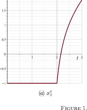
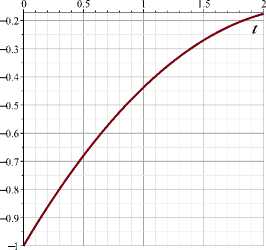
( b ) x ^c2

State variables

Table 1. Results of a first-order method

Iteration Functional I

0           1.98

1           1.85

The functional is I = x C (3) ^ min.

Construct the DCS system. It is easy to see that K = 0,1, 2. Since x 1 is a linking variable in the two periods under consideration, we can write a process of the upper level in terms of this variable

x(0) = x 1 (0, 0) = -1,        x(1) = x 1 (0, 2), x(2) = x 1 (1, 3),

I = x(2),               x 1 (1, 2) = x(1),            e = x(1).

The basic constructions have the form:

H ^c (0, t, x 1 ,x 2 ,u, <, ^ c ) = < ((x c ) 2 (x 2

u)

2 ) + ^ c ^1 X 2 + 3u 3) ,

H ^c (1, t, x 1 ,u, ^ C ) = ^ C ((x C - t) ² + u ² ) .

In [11] , we have found the solution using the first-order method with initial u I = 0.5, I I = 1.98. The results are given in Figires 1, 2 and Table 1.

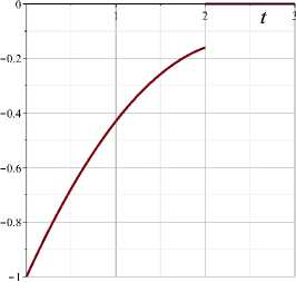
Figure 2. Control u

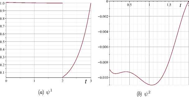
Figure 3. Vector ψ ^c

Let us verify that the solution obtained provides a relative minimum of the functional I . Since the solution is numerical, the function Hc and its first and second derivatives are also numerical. By virtue of the fact that the equations of every stage do not depend on the variable x of the upper level, we have A = 0, в = 0, ш = ^cT = (^C, ^c)T and

0. It is easy to see that at stage 1

- c = /^1  'ч Л .

σ 21   σ 22

The results displayed in Figures 3 –4 show that the system of vector-

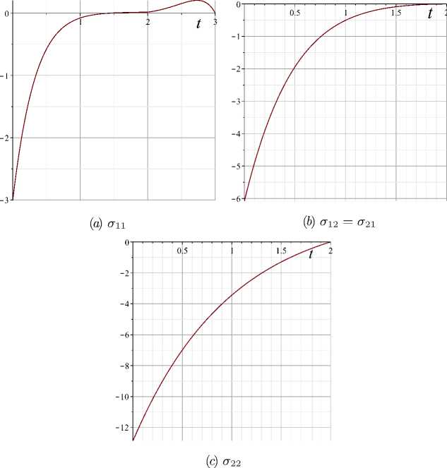
Figure 4. Matrix ac matrix differential equations for ψc , σc has the solution in both stages.

Therefore, m provides a relative minimum of the functional.

Conclusions

In this paper, we derive sufficient relative minimum conditions for discrete-continuous systems. It allows us to verify that the proposed solution of the optimal control problem provides a local minimum for the functional. An illustrative example is provided.