Support Vector Machine as Feature Selection Method in Classifier Ensembles

Published Online April 2014 in MECS DOI: 10.5815/ijmecs.2014.04.01

A process that chooses a minimum subset of M features from the original set of N features, so that the feature space is optimally reduced according to a certain evaluation criterion can be defined as feature selection. Finding the best feature subset is usually intractable and many problems related to feature selection have been shown to be NP-hard.

Feature selection is an active field in computer science and it has been a fertile field of research and development since 1970’s in statistical pattern recognition machine learning and data mining. It is a fundamental problem in many different areas, especially in forecasting, document classification, bioinformatics, and object recognition or in modelling of complex technological processes. In such applications, datasets with thousands of features are not uncommon and for some problems all features may be important, but for some target concepts, only a small subset of features is usually relevant.

Various aspects of feature selection have been studied. Search is a key topic in the study of feature selection [1] such as search starting points, search directions, and search strategies. Another important aspect is how to measure the goodness of a feature subset [2]. Algorithms for feature selection may be divided into filters [2, 3], wrappers and embedded approaches [4]. Filters methods evaluate quality of selected features, independently from the classification algorithm, wrapper methods require application of a classifier to evaluate this quality, while embedded methods perform feature selection during learning of optimal parameters. According to class information availability in data, there are supervised feature selection approaches as well as unsupervised feature selection approaches.

Some classification algorithms have inherited ability to focus on relevant features and ignore irrelevant ones. Decision trees are primary example of a class of such algorithms, but also multi-layer perceptron neural networks, with strong regularization of the input layer, may exclude the irrelevant features in an automatic way [5]. Such methods may also benefit from independent feature selection. On the other hand, some algorithms have no provisions for feature selection. The k-nearest neighbour algorithm is one family of such methods that classify novel examples by retrieving the nearest training example, strongly relaying on feature selection methods to remove noisy features.

The main aim of this paper was to experimentally verify the impact of SVM as feature selection method on classification accuracy with classifier ensembles. We use classifier ensembles, instead of individual classifier, because in many fields, multiple classifier system is more accurate and robust than an excellent single classifier.

In this study, we suggest classifier ensembles that can incorporate SVM as feature selection method into classifier ensembles models. The goal of this research is also to present and compare different algorithmic approaches for constructing and evaluating systems that learn from experience to make the decisions and predictions and minimize the expected number or proportion of mistakes.

The paper is organized as follows. In the next section we briefly described general issues concerning SVM. Section 3 gives a brief overview of adopted algorithms, namely, Bagging, AdaBoost, Rotation Forest, Dagging, Decorate, MultiBoost and LogitBoost. Section 4 discusses the results and investigates the performance of the proposed technique. Finally, concluding remarks are discussed in section 5.

• II.    Support Vector Machine

Various feature ranking and feature selection techniques have been proposed in the machine learning literature, which purpose is to discard irrelevant or redundant features from a given feature vector. In this paper, we consider evaluation of the practical usefulness of SVM as feature selection technique on classification accuracy with classifier ensembles, as filter method which evaluate each subset.

SVM introduced by Vapnik [6], employs structural risk minimization whereby a bound on the risk is minimized by maximizing the margin between the separating hyperplane and the closest data point to the hyperplane. SVM as supervised learning methods that analyze data and recognize patterns, rigorously based on statistical learning theory simultaneously minimizes the training and test errors.

In 1963 Vapnik proposed original optimal hyperplane algorithm, which was a linear classifier, but often happens that in a finite dimensional space the sets to be discriminated are not linearly separable. In 1992, Boser, Guyon and Vapnik [7] suggested a way to create nonlinear classifiers by applying the kernel trick (originally proposed by Aizerman, Braverman and Rozonoer [8]) to maximum-margin hyperplanes. In this algorithm, every dot product is replaced by a nonlinear kernel function, which allows the algorithm to fit the maximum-margin hyperplane in a transformed feature space. To make the separation easier, it was proposed that the original finite-dimensional space be mapped into a much higher-dimensional space. Mapping into a larger space, cross products may be computed easily in terms of the variables in the original space, making the computational load reasonable.

SVM constructs a hyperplane or set of hyperplanes in a high dimensional space, which can be used for classification, regression, or other tasks. Many hyperplanes might classify the data; the best hyperplane is the one that represents the largest separation, or margin, between the classes. Generally, the larger the margin it is the lower the generalization error of the classifier. We choose the maximum–margin hyperplane, such the hyperplane in which the distance from it to the nearest data point on each side is maximized.

SVM is explained below. Given training vectors xj ϵR n,i = 1,…,l , in the two-class case and the corresponding class labels decision yjϵ{1, -1} ,the statement of SVM optimization for classification problems may be the following [9, 10]:

min w,b, ^2wTw+С∑i=l ξi (1)

with constraints: yi (w T ϕ(xi)+b)≥1-ξi, ξi≥0,i= 1,…, . The dual problem definition is:

min∝ ∝ T Ԛ∝-еT∝, 0≤∝i≤С,i=1,…,l, (2)

with constraints y T ∝= 0, where e is the vector of all ones, C > 0 is the upper bound, Q is a l by l positive semi definite matrix, Qij ≡уiyj K(xi,xj ), and K(xi,xj)≡ ϕ(x j )T ϕ(xj ) is the kernel. Function Ф transforms training vectors Xj into a higher (maybe infinite) dimensional space. The decision function is sgn(∑^iVt ∝tK(xt ,X)+b) (3)

The choice of kernel results in different kinds of SVM with different performance levels. The choice of the appropriate kernel for a specific application is often a difficult task. A necessary and sufficient condition for a kernel to be valid is that it must satisfy Mercer’s theorem, but other than that, there is really no mathematically structured approach to prefer one kernel to the other.

• III.    Classifier Ensembles

In machine learning and pattern recognition, in many fields multiple classifier system is more accurate and robust than an excellent single classifier, because one single classification system cannot always provide high classification accuracy. Classifier combination is an active field of research for the reason that a lot of theoretical and practical studies present the advantages of the combination paradigm over the individual classifier models. A great deal of study has gone into designing multiple classifier systems that are commonly called classifier ensembles. Seven approaches for constructing classifier ensembles are presented, which have been found to be accurate and computationally feasible across various data domains.

• A.    Bagging

  The Bagging predictor firstly was introduced in 1996 by Breiman [11], who shows in his work that the Bagging predictors can push an unstable weak classifier to a significant step towards optimality. Bagging [11] takes bootstrap samples of objects and trains a classifier on each sample. The classifier votes are combined by majority voting. In some implementations of Bagging, classifiers produce estimates of the posterior probabilities for the classes. Posterior probabilities are averaged across the classifiers and the most probable class is assigned, called “average” aggregation of the outputs.

For- к = 1, 2,..., K-Do*1

And form the learning set L^.^

Train - classification yk- (L (д)- йот the-learning -set L^ .• Make a plurality ■ vote-for every qok of К classifications on thetest-set.+J

The classification, which- gets the most -voting- score, is ■ the best one.*'

Fig.1. Bagging algorithm [12]

Bagging with average aggregation is used in this experiment. Each individual classifier is trained on a bootstrap sample, which causes the data distribution seen during training is similar to the original distribution. Therefore, the individual classifiers in a bagging ensemble have relatively high classification accuracy.

Only the proportion of different objects in the training samples encourages diversity between these classifiers. The bootstrap sampling appears to lead to ensembles of low diversity compared to other ensemble creating methods, even though the classifier models used in Bagging are sensitive to small changes in data. For that reason, Bagging requires larger ensemble sizes to perform well.

Bagging algorithm is showed in Fig. 1. A learning set consists of data L ≔ {(yn,xn), n = 1,2,…, N}, where xn ∈ X is the input and y n ∈ Y is the response from a predictor denoted by φ(Χ, L). Suppose we are given k learning sets {Lк} of N independent identical distribution observation from the same distribution of L. An obvious procedure to use the average to get a better estimate of the classification:

Фа (X)=El Ф (X,L) (4)

where EL denotes the expectation over L . Generally, we only have one learning set L , so, one resolvable way is to take bootstrap samples { L ( g ) } of N ( g ) cases, randomly, but with replacement from L , and form predictor set { Ф ( X , L ( g ) )} . This procedure is called “bootstrap aggregating” and use the acronym Bagging. In that case, the predictor φ , which gets most voting score of test set, is the best classification.

• B.    AdaBoost

Boosting is a family of methods for improving the performance of a “weak” classifier by using it within an ensemble structure, the most prominent member of which is AdaBoost. In Boosting methods, a set of weights is maintained across the objects in the data set, so that objects that have been difficult to classify acquire more weight, forcing subsequent classifiers to focus on them. Mechanism of these methods consist of repeatedly running a given weak learning algorithm on various distributions over the training data, and then combining the classifiers produced by the weak learner into a single composite classifier.

The Boosting algorithm takes as input a training set of m examples S = 〈 (x^ ,y ^),…,(xm,ym) 〉 where xi is an instance drawn from some space X, and yi ∈ Ү is the class label associated with xi. In this research, is assumed that the set of possible labels Y is of finite cardinality k. The Boosting algorithm calls weak learning algorithm repeatedly in a series of rounds. On round t, the booster provides weak learning algorithm with a distribution Dt over the training set S. Weak learning algorithm computes a classifier or hypothesis hypothesis h_t:Х → Ү, which should misclassify a non trivial fraction of the training examples, relative to Dt. The goal of weak learner is to find a hypothesis ht that minimizes the training error ϵ_t = Pri_~ Dt [h_t (x i)≠yi]. Training error is measured with respect to the distribution Dt that was provided to the weak learner. This process continues for

T rounds. At last, the booster combines the weak hypotheses h^ ,…,hT into a single final hypothesis h fin . In the Boosting algorithm the manner in which Dt is computed on each round, and how h fin is computed are unspecified and these questions solve different Boosting schemes in different ways.

AdaBoost.M1 algorithm uses the simple rule present in Fig. 2, where the initial distribution D1 is uniform over S so D1(i)=1/m for all i. In this algorithm to update distribution, the weight of example i is multiplied by some number β_t ∈ [0,1] if ht classifies xi correctly, and otherwise the weight is left unchanged, and also divide by the normalization constant Zt. Thus, “hard” examples, which tend often to be misclassified, get higher weight, and “easy” examples that are correctly classified by many of the previous weak hypotheses get lower weight. Accordingly, AdaBoost.M1 focuses the most weight on the examples that seem to be hardest for weak learning algorithm.

Input: sequence of m examples ((x₁,y₁),...,(x_m,y_nl)) withlabels-y_£ e У = {1, ...,к}^

weak learning algorit hm )-¹

integer-T'specifyingnumber of iterations^1

Initialize Di(i)—l/m for all- i.^

Do for t = 1,2, ...,7k-

• 1 .-«Call-weak learning algorithm, providing it with the-distribution D_t^

• 2 .-«Get back hypo thesis h_t:X —> Y.v

• 3 .-«Calculate the error of h_t : e_t = 2_!;а_г(х,)ху_г ^r (O '

• 5 .^Update distribution D_f: ^_t+1(0 = —— X

If e_t >  1/2, then set Г = t — 1 and abort 1оор>

4,-Set p_t = e_t/(l - e_t)^

№t if ^г(^) = Yi^

11 otherwise where Zt is a normalization constant (chosen so that

Dc+1 -will be a-distribution).*1

Output the final hypothesis: -

^tnGO = argmaxSt;ht(,)=yZoS^.

Fig.2. AdaBoost.M1 algorithm [13]

The number βt is a function of ϵt and the final hypothesis h fin is a weighted vote of the weak hypotheses. The weight of hypothesis ht is defined to be ln1/βt so that greater weight is given to hypotheses with lower error.

The success of AdaBoost algorithm has been explained, among others, with its diversity creating ability, which is an important property of a classifier ensemble [14]. This algorithm creates inaccurate classifiers by forcing them to concentrate on difficult objects and ignore the rest of the data, which led to large diversity that boosted the ensemble performance, often beyond that of Bagging. This leads us to the famous accuracy-diversity dilemma, because it seems that classifiers cannot be both very accurate and have very diverse outputs.

• C.    Rotation Forest

Rotation Forest is an ensemble method that trains classifiers independently, using a different set of extracted features for each of classifier, which is accurate and feasible across various data domains [15].

Rotation Forest randomly split the feature set into K subsets, which a base classifier uses as training data, and chose disjoint subsets to maximize the chance for high diversity. The filter used to project the data applied to each subset. Running the filter on a subset of classes instead of the whole set is done in a bid to avoid identical coefficients if the same feature subset is chosen for different classifiers.

Details about Rotation Forest algorithm are presented below. Assume that there are N training samples and n features in data set. Let X be the training sample set in a form of a N × n matrix, Y be the corresponding labels, where Y takes values from the set of class labels {W_T,…,W_c}, and F be the feature set. Assuming there are L decision trees in Rotation Forest, denoted by D1,..., DL respectively, and the feature set split randomly into K subsets, we need to determine L and K in advance.

Training Phase

Given*

• • aining data set-(an N X n matrix)*

• • •У: the labels of the tr ainin g set (an N X 1 matrix)*

• • *£: the numb er ■ о f -clas si fi ers in - the -ens emble

• •*£: the numb er ■ о f sub s et s

• • [к*], .... w_c} the set of-class-labels*

Fori = 1 ... L

••Prepare the rotation matrix 7?“:*

oiSplrt F^the featme set)into71 subsets: Fjj(for-

oForj = 1... Kv

• ■    Let JYybethedataset JTforthefeatmesinFij

• ■    Elimin at e - from X_ua rand om -sub s et - о f clas s es*

• ■ ♦S elect -a-bо ot strap 'sample ■ from Хц.о f-size 7 5%-o f the numb er ■ о f obj ect s in Xy. -D enot e the new s et ■ brXj*

•♦Apply PCA ■ on X_{t j} to ■ obtain the- coefficients in a matrix С_г ■*

o Arrange the C, -for 7=1... К in a rotation matrix /?*

oConstruct Я° Ьу rearranging the columns of flj to-matchthe order of features in F.*

••Build classifier- Dousing (XR°,y) as the training set*

Classification Phase

••Fora-given-x,-let ■d_j-(xfl°)-be-the-probability produced by -the classifier D, to thehypothesis that x belongs to class Wj. By the average combinationmethod, calculatethe confidence-for-each class as follows:*

L

Hjto = ^^ d_{t j} (xR^J = 1,.... c

The-test - s am pie-x is - easily assigned-to the- class-with-the largest-confidence.J

Fig.3. Rotation Forest algorithm [15]

Construction of the training set for an individual classifier Di is in three steps. In step1, split F randomly into K disjointed subsets. Suppose that K is a factor of n so that each feature subset contains M=n⁄K features. In step 2, denote by Fij the jth subset of features for training set of classifier Di. Select randomly for each subset, a nonempty subset of classes, and then draw a bootstrap subset of objects with the size of 75 percent of the data set to form a new training set. After that, PCA is applied to the M features in Fij and the selected subset of X. Denoted the coefficients of PCA by a( ),…,a(Mj ) each of

,J ' ' 1,J size M×1. In step 3, arrange a sparse rotation matrix Ri with the obtained coefficients. The columns of Ri should be rearranged according to the original features and the rearranged rotation matrix is denoted by R f . The transformed training set for classifier Di is ХR f . All classifiers will be trained in parallel. In the classification phase of Rotation Forest, for a given x, let d , (xR t ) be the probability produced by the classifier Di to the hypothesis that x belongs to class wj . By the average combination method, calculate the confidence for each class as follows:

^j (X)= 7 ∑i=i ^i,j(xR^), j=1,…,c (5)

The test sample x is easily assigned to the class with the largest confidence. The algorithm of Rotation Forest is showed on Fig. 3.

• D.    Dagging

Ting and Witten [16] introduced Dagging as ensemble method, which is very similar to Bagging, but instead of using bootstrap sampling it uses disjoint samples. The training set is partitioned into K subsets, and a base classifier generates a hypothesis for each subset. The final prediction is done with plurality vote as in Bagging. A further difference is Dagging uses no extra resources, since the same amount of examples are used as the training set. This ensemble method is useful for base classifiers that are quadratic or worse in time behavior, regarding number of instances in the training data.

In his research Ting and Witten were tested Bagging and Dagging with C4.5, considered unstable classifier, and Naive Bayes, considered stable classifier. Although Breiman reports that Bagging doesn’t generally work well on stable classifiers, Ting and Witten conclude that Bagging as well as Dagging, do well on both unstable and stable algorithms.

• E.    Decorate

Decorate directly constructs diverse hypotheses using additional artificially-constructed training examples [17]. The diversity of an ensemble of classifiers is known to be an important factor in determining its generalization error. This classifier ensemble can use any strong learner (one that provides high accuracy on the training data) as a base classifier to build diverse committees.

In Decorate (Fig. 4), an ensemble is generated iteratively, first learning a classifier and then adding it to the current ensemble. The ensemble is initialized to contain the classifier trained on the given training data. In successive iteration, the classifiers are trained on the original training data combined with some artificial data. In iteration, artificial training examples are generated from the data distribution; where the number of examples to be generated is specified as a fraction, Rsize, of the training set size. The labels for these artificially generated training examples are chosen so as to differ maximally from the current ensemble's predictions. A new classifier is trained on the union of the original training data and the diversity data, thereby forcing it to differ from the current ensemble. As a result, adding this classifier to the ensemble should increase its diversity. To maintain training accuracy, a new classifier is rejected if adding it to the existing ensemble decreases its accuracy. Decorate is repeated this process until the desired committee size or exceed the maximum number of iterations are reached.

combination may be able to retain AdaBoost’s bias reduction while adding Bagging’s variance reduction to that already obtained by AdaBoost.

The resulting MultiBoost algorithm is presented in Fig. 5. This algorithm besides the bias and variance reduction properties that may inherit from each of its constituent committee learning algorithms, has the potential computational advantage over AdaBoost that the subcommittee may be learned in parallel, although this would require a change to the handling of early termination of learning a sub-committee. The AdaBoost process is inherently sequential, minimizing the potential for parallel computation, but each classifier learned with Wagging is independent of the rest, allowing parallel computation, a property that MultiBoost inherits at the sub-committee level.

Input:*

BaseLearn - base-learning algorithms

T -■ set- of- m training examples < (x₁,y₁), .../(^„.y^,)^-with lab els y^eY

C_Zn, - desired-ensemble- sizes

Диг - maximum number of iterations to build an ensemble*' R^, -- factor that determines number of artificial examples to-gen crates i= 1 ' trials = 1 s

Cf—BaseLearnfT)*1

Initialize ensemble.- C* = {Cj}s

Compute ensemble enor. e = —4----4——*'

While! < C_Sn_e an.& trials <1,^

Generate- R_size X |T| tr ainin g examples, R, based on-distribution of training data*

Label examples in R-with-probability of class labels invers ely -proportional t о -predicti ons - о f C^{8 J} T = TUH -* s

C' ■ = BaseLeamiT;

C8 = C* U{C3s

T = T — R.removetheartificialdatas Computetraining error, 6, ofC‘s Ife < e 1=1 + 1"S e = e p otherwise. ¹ C⁸ =C⁸- {C^s trials = trials + Is

Fig.4. Decorate algorithm [17]

• F.    MultiBoost

MultiBoost is technique for combining Boosting and Wagging (which is in turn a variant of Bagging). Bagging and AdaBoost appear to operate by diverse mechanisms, have different effects, and both have greatest effect obtained from the first few committee members, which suggest that it might be possible to obtain benefit by combining them. Because the mechanisms are differing, their combination may out-perform either in isolation. AdaBoost reduces both bias and variance and Bagging mainly reduces variance, but more effective than AdaBoost at reducing variance. It is reason why their

Input:s

S,- a- sequence of m labeled- examples «Лг-уД-, (^_т,Ут) > with labels?^ P> base learning algorithm BaseLearn.s integer 7specifying the numberofiterations.* vector of integers It specifying the iteration at which each subcommittee i > 1 should* terminate.*¹

S'~S with instance-weightsassignedto be 1 .s set k- l.s

For r= 1 to 7{*'

If It=t then*¹

reset- S'- to random wei^its drawn from the continuous Poisson distribution.*1

standardize-S '-to -sum to и.*1

increment A:.*1

Ct ^BaseLearn^X.Step 8).*¹

standardize-S'to sum to и.*1

increment A.*1

go to Step 8.*1

otherwise if £t = 0 then*

set Д to 10"10*1

reset- S'- to random wei^its drawn from the continuous Poisson distribution.*1

standardize-S' to sum to и.*1

increment A.*1

otherwise,^

For each jc, eS',*'

divide waqg/i^ybyZSt if C^cj) * у_} and 2(1 - е[)- otherwise.*¹

if weight(xj) <  10 ®, set wergfe(j9) to 10"® -*¹

Output the final classifier:*¹

0^) = ”^,^ , lo_S-.'

Fig.5. MultiBoost algorithm [18]

• G.    LogitBoost

LogitBoost performs classification using a regression scheme as the base learner, and can handle multi-class problems (Fig. 6). This classifier ensemble can do efficient internal cross-validation to determine appropriate number of iterations.

Start with wei ghts шц = 1/N,i = l,...,N,j = l,-,J,Fj (x) = 0 and

Pjto = 1/JVj^

Repeat form = 1,2,..., M:^

• (a)    Repeat for j = 1, ...J:^

• (i)    Compute working responses and weights in the /th classy

_ Уц-PjtxD

Zy pjUtXi-PjUt>y соо=р,(х^)(1 -pjCx^y^

(ii)- Fit the function ^-f_mj(x) by a weighted leastsquares regression ofz^to-Xi with wei^itsm^.tJ

• (b)    Set f_mj (x) <- ^ (J_mj to - jSLi fmk to). anfi

Fj to «- Fj to + frnj to -^

• (c)    Update-p_; (x)-^

Output the classifier argmaxyfjCx).^

Fig.6. The LogitBoost (J classes) algorithm [19]

• IV.    Outcomes of Undertaking Coursework

In this section, we will investigate the impact of data dimensionality reduction with SVM on classification accuracy with classifier ensembles. Consequences of choosing different number of features are monitored. Later on, comparisons of results of measuring the performance of classifiers are presented. For the purpose of this research, SVM classifier evaluates the worth of each feature. Features are ranked by the square of the weight assigned by the SVM [20]. The WEKA toolkit is used to analyze the dataset [21, 22].

Five real data sets in medical domains were used for tests, taken from the UCI repository of machine learning databases [23]. We used these data sets to compare results of classification with data dimensionality reduction by SVM in medical diagnosis.

To achieve the goal of classifier ensemble to produce a model (based on the training data) which predicts the target values of the test data given only the test data features; the following procedure is used. It consists of transform data to the appropriate format, conduct simple scaling on the data, use linear kernel K(x j , X j ) = x ^ for feature selection, and finally use one of the classifier ensembles for classification. We set classifier ensembles in following way:

• •    AdaBoost.M1 algorithm is used, which use the base classifier DecisionStump and reweighting, the number of iterations is set on 10, and weight threshold for weight pruning is set on 100.

• •    Bagging use the base classifier REPTree, size of each bag, as a percentage of the training set size is

set on 100, the out-of-bag error is not calculated, the number of iterations is set on 10.

• •    Rotation Forest use the base classifier J48, the number of iterations is set on 10, the filter used to project the data is set on Principal Components, and the percentage of instances to be removed is set on 50.

• •    Dagging use the base classifier SMO (John Platt's sequential minimal optimization algorithm for training a support vector classifier) and the number of folds to use for splitting the training set into smaller chunks for the base classifier is set on 10.

• •    Decorate use the base classifier J48, the desired number of member classifiers in the Decorate ensemble is set on 10 (larger ensemble sizes usually lead to more accurate models, but increases training time and model complexity) and the maximum number of Decorate iterations to run is set on 10.

• •    MultiBoostAB use the base classifier Decision Stump and reweighting, the number of iterations is set on 10, the number of subcommittees is set on 3, and weight threshold for weight pruning is set on 100.

• •    LogitBoost use the base classifier Decision Stump and reweighting, threshold on improvement in likelihood is set on -1.798E308, no cross-validation is performed, and the number of iterations is set on 10.

The experiment was first unleashed the ranking of importance of each feature in the data sets. Dimensionality reduction was done by reduced number of features in each data set; taking into account that the feature which has the lowest significance is first rejected. Then, the classification accuracy is measured by applying different classifier ensembles. Classifier ensembles were used for the good performance shown by the preliminary study, the high classification accuracy and high speed operation. After that, was analyzed the effect of reducing the number of features on the accuracy of each classifiers.

Our implementation is as follows. The training data is separated into 10 subsets of equal size in 10-fold crossvalidation. Sequentially one fold is considered as the validation set and the rest are for training. The cross validation accuracy is the average of accuracy on predicting the validation sets. Results of classification accuracy, as a method for measuring the performance of SVM for five data sets in medical domains, are presented on Fig. 7, Fig. 8, Fig. 9, Fig. 10 and Fig. 11. Selecting appropriate features for a given data set, the reliability of classification for most of data sets and classifier ensembles is increased.

For Pima data set, with all classifier ensembles algorithms, using the SVM for feature selection, we get at least the same or higher classification accuracy. In most cases, five of seven cases, the greatest classification accuracy were achieved with five features, instead of the eight features as it was in the original data set. For Pima data set, maximum improvement of the classification accuracy with SVM as feature selection method, compared to the classification accuracy without selection of features is as follows: AdaBoost is 1.56%, Bagging is 0.52%, Rotation Forest is 1.17%, Dagging without improvement, Decorate is 2.6%, MultiBoostAB without improvement and LogitBoost is 1.04%.

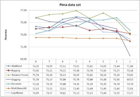
Fig.7. Pima data set and impact of selected features on classification accuracy

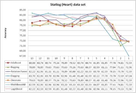
Fig.8. Statlog(Heart) data set and impact of selected features on classification accuracy

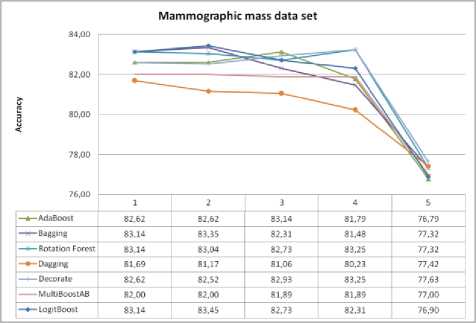
Fig. 9. Mammographic mass data set and impact of selected features on classification accuracy

In the case of Statlog (Heart) data set, for all algorithms, using the SVM for feature selection method, we get at least the same or higher classification accuracy. In all cases except in one case, the highest classification accuracy was achieved with five features, instead of the thirteen features as it was in the original data set. For

Statlog (Heart) data set, maximum improvement of the classification accuracy with SVM as feature selection method, compared to the classification accuracy without selection of features is as follows: AdaBoost is 1.85%, Bagging is 3.7%, Rotation Forest is 1.48%, Dagging without improvement, Decorate is 1.85%, MultiBoostAB is 1.48% and LogitBoost is 0.74%.

In the case of Mammographic mass data set, in all algorithms, using the SVM for feature selection method, we get at least the same or higher classification accuracy, except for Dagging classifier ensembles which leads to less accuracy of classification. In three cases of seven cases, classification accuracy was achieved with four features, instead of the five features as it was in the original data set. For Mammographic mass data set, maximum improvement of the classification accuracy with SVM as feature selection method, compared to the classification accuracy without selection of features is as follows: AdaBoost is 0.52%, Bagging is 0.21%, Rotation Forest is 0.11%, Dagging without improvement, Decorate is 0.63%, MultiBoostAB without improvement and LogitBoost is 0.31%.

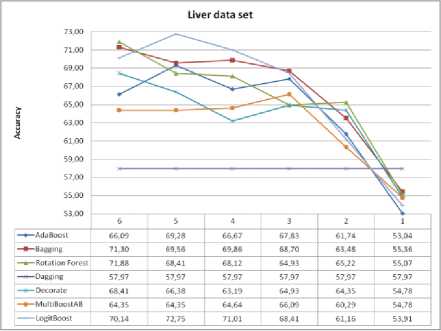
Fig.10. Liver data set and impact of selected features on classification accuracy

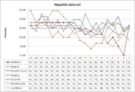
Fig.11. Hepatitis data set and impact of selected features on classification accuracy

For Liver data set, in all algorithms, using the SVM for feature selection method, we get at least the same or higher classification accuracy, except for Bagging, Rotation Forest and Decorate classifier ensembles. In three cases of seven cases, the classification accuracy was achieved with five features, instead of the six features as it was in the original data set. For Liver data set, maximum improvement of the classification accuracy with SVM as feature selection, compared to the classification accuracy without selection of features is as follows: AdaBoost is 3.19%, Bagging without improvement, Rotation Forest without improvement, Dagging without improvement, Decorate without improvement, MultiBoostAB is 1.74% and LogitBoost is 2.61%.

For Hepatitis data set, for all algorithms, using the SVM for feature selection method, we get at least the same or higher classification accuracy, except for Decorate classifier ensembles. The largest classification accuracy was achieved with different numbers of features. With the decrease of the number of features, the classification accuracy of some algorithms oscillates around some value. For this data set, with a very small number of selected features, high classification accuracy was achieved. For Hepatitis data set, maximum improvement of the classification accuracy with SVM as feature selection method, compared to the classification accuracy without selection of features is as follows: AdaBoost is 0.65%, Bagging is 2.58%, Rotation Forest is 1.29, Dagging is 2.58%, Decorate without improvement, MultiBoostAB is 1.29% and LogitBoost is 0.64%.

• V.    Conclusion

This paper investigates the impact of feature selection with SVM on classification accuracy with classifier ensembles. Classifier ensembles with SVM as feature selection method has used on five medical data sets. These results evaluated and compared choosing different number of selected features. Experimental results demonstrate the effectiveness of selecting features with SVM in various types of classifier ensembles.