Synergy of Schur, Hessenberg and QR Decompositions on Face Recognition

Author: Jagadeesh H S, Suresh Babu K, K B Raja
Journal: International Journal of Image, Graphics and Signal Processing(IJIGSP) @ijigsp
Article in issue: 4 vol.8, 2016.
Free access
Human recognition through faces has elusive challenges over a period of time. In this paper, an efficient method using three matrix decompositions for face recognition is proposed. The proposed model uses Discrete Wavelet Transform (DWT) with Extended Directional Binary codes (EDBC) in one branch. Three matrix decompositions combination with Singular Value Decomposition (SVD) is used in the other branch. Preprocessing uses Single Scale Retinex (SSR), Multi Scale Retinex (MSR) and Single scale Self Quotient (SSQ) methods. The Approximate (LL) band of DWT is used to extract one hundred EDBC features. In addition, Schur, Hessenberg and QR matrix decompositions are applied individually on pre-processed images and added. Singular Value Decomposition (SVD) is applied on the decomposition sum to yield another one hundred features. The combination EDBC and SVD features are final features. City-block or Euclidean Distance (ED) measures are used to generate the results. Performance on YALE, GTAV and ORL face datasets is better compared to other existing methods.
City-block distance, Euclidean distance, Extended directional binary codes, Matrix decomposition, Singular value decomposition
Short address: https://sciup.org/15013971
IDR: 15013971
Text of the scientific article Synergy of Schur, Hessenberg and QR Decompositions on Face Recognition
Published Online April 2016 in MECS and Computer Science
Smart verification and recognition of objects in any scenario is elusive. Methods adopted for recognizing the objects are made automated timely as applied to many areas including in industries [1], social security or consumer electronics. The transformation occurred during the decade back that the machines / robots replacing the humans for many services. From object to human recognition, the technology uses different metrological [2] parameters. Human recognition systems has major role in many real time situations. Various proposed methods by many researchers have bounded solutions. Biometric solutions are the remedy for many subtle issues compared with conventional ways. Human body consists of many distinct physical structures such as some sense organs, hand, face and voice, gait, expression are few behavioral traits. These biometric parameters are used either individually or in combined manner in various applications. The real time implementation methods are classified based on features and images [3]. The feature based method extracts attributes from components of an image e.g. eyes, nose, mouth and other parts of face, but image based methods considers different regions or structures of image. The smile expression recognition [4] is becoming indispensible to interact with computers. In spite of illumination, occlusion, pose variations during image acquisition, the range or distance [5] also affects the image quality and performance of the system. When an input image is degraded or corrupted by noise from any means, it is corrected and improved in quality by preprocessing [6]. Remaining steps of declaring results of a system includes; dimension reduction / feature extraction and comparison. Many researchers work for improving the recognition performance by proposing new tools and techniques for preprocessing, feature extraction and matching. The real time implementations require resources with high computational capacity [7] in law enforcement applications. Face recognition accuracy is influenced by number of images used for training, image size and number of classes. Digital signal processors [8] cater the hardware implementation of face recognition systems from video input. Execution time of algorithms should be as less as possible to cope up with the varying constraints. Faster algorithms are developed by reducing the dimension of data e.g. Principal Component Analysis (PCA), Fisher’s Linear Discriminant (FLD) [9], Discrete Cosine Transform (DCT), Discrete Wavelet Transform (DWT) and Singular Value Decomposition (SVD). Other approaches using descriptors such as Local Binary Patterns (LBP) [10] and Directional Binary Codes (DBC) [11] are proposed for textures and edge information extraction respectively.
The remainder of this paper is organized as follows. Section II reviews the necessary literature survey. The proposed MDE – D3S FR model is explained in Section III. Algorithm of the proposed work is discussed in section IV. Performance is analyzed in section V and concluded in section VI.
-
II. Related Work
Zheng-Hai Huang et al., [12] proposed two feature extraction methods for face recognition by pixel and feature level fusion. It uses top level wavelet sub bands in combination with Principal Component Analysis (PCA) and Linear Discriminant Analysis (LDA) for fusion. The proposed scheme is robust on FERET, ORL and AR face databases. Shahan Nercessian et al., [13] introduced parameterized logarithmic dual tree complex wavelet transform and its application to image fusion. It is a nonlinear way of processing images in image processing framework used for image analysis. The results are qualitatively and quantitatively better compared to other fusion algorithms.
Aruni Singh and Sanjay Kumar Singh [14] addressed face tampering effect on four face recognition algorithm categories. Accuracy of each algorithm is varying and unpredictable. Performance is tested on PIE, AR, Yale B and their own face databases. It is concluded by developing a gradient based method for face tampering detection. Chung-Hao Chen et al., [15] proposed an automated method for computer based face recognition for surveillance application. It can be used for customized sensor design with given illuminations. The Pan Tilt Zoom (PTZ) cameras used covers panoramic area and yield high resolution images. Mapping algorithm derives the orientation between two PTZ cameras and relative positioning using unified polynomial model. Experimental results prove the reduction in computational complexity by improving flexibility.
-
III. Proposed Algorithm
The details of the work proposed is discussed in this section. The algorithm consists of steps such as Preprocessing, DWT, EDBC [16], Matrix decompositions, SVD and Matching to yield the results. Figure 1 shows the block diagram of the proposed DWT - EDBC and three Decompositions with SVD based Face Recognition (MDE – D3S FR) model.
-
A. Databases
Three publically available Yale, GTAV and ORL face databases are used to test the performance.
-
(i) YALE database [17] consists of totally 165 Graphics Interchange Format (GIF) images of 15 individuals, with 11 images per subject. Each image has variation in facial expressions or configurations such as left-light, center-light, right-light, wearing glasses, without wearing glasses, neutral, happy, sleepy, surprised, sad, and wink. All images are with dimension 243*320 and 24 bit pixel depth. The pixels are arranged with 96 dpi. The GIF is converted to JPEG in our work.
-
(ii) GTAV (Audio Visual Technologies Group) Face database [18], has been created for the purpose
of evaluating robustness of any face recognition algorithm over illumination and pose variations. It includes total 44 persons with 27 images per person. Many images are captured under three different illuminations such as light source at an angle 45º, natural light, and frontal strong light source. Other few images are acquired at 0º, ations.
Remaining images are captured with different facial expressions and occlusions. Resolution of each image is 240*320 and all are in Bit Map (BMP) format. The pixel depth is 24 bits.
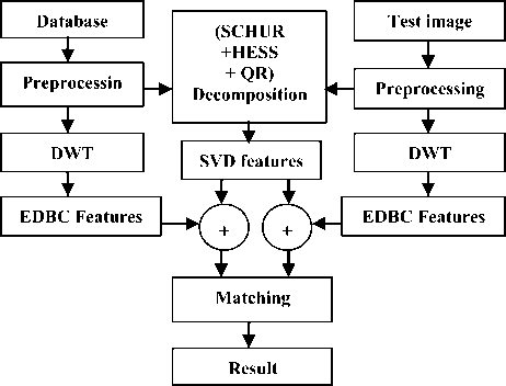
Fig.1. Block Diagram of the Proposed MDE – D3S FR Model
-
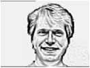
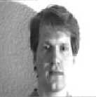
(iii) The ORL face database [19], has a total of 400 images of 40 different subjects. Ten images per person are acquired at different times by varying lighting intensities. Different facial expressions such as smiling or non-smiling face and images with opening or closing of eyes are acquired. It includes facial images of wearing glasses or without wearing glasses also. All the subjects are in frontal, up-right position with a dark homogeneous background. All images have 92*112 size and represented by 8-bit grey levels in JPEG format. Each image has 96 dpi of horizontal and vertical resolution. Figure 2 shows the one sample image each of Yale, GTAV and ORL face database.
-
B. Pre-processing
Three methods out of fourteen Illumination Normalization techniques for robust Face recognition (IN-Face) toolbox [20], [21] are used to perform preprocessing. Single Scale Retinex (SSR) algorithm, Multi Scale Retinex (MSR) algorithm and Single scale Self Quotient image (SSQ) are used to process input images in the proposed work.
-
(i) SSR algorithm [22] is based on Retinex theory [23], which uses flux independent image representation. The word Retinex is a combination of words Retina and Cortex. It
computes lightness values for each pixel in the image and uses thresholding operation to reduce the non-uniform illumination effects. Retinex theory has the major advantage of representing the image details independent of ambient light`s spectral power distribution and surface reflectance of the objects in a scene.
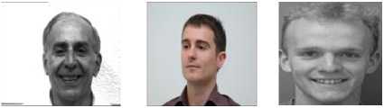
(a) YALE database (b) GTAV database (c) ORL database
Fig.2. Image Samples of Three Face Databases
-
(ii) MSR algorithm [24] is an extension of SSR algorithm, both uses the Gaussian smoothing filters. The default sizes of Gaussian filters are 15 and [7 15 21] for SSR and MSR respectively.
-
(iii) Self-Quotient Image (SQI) [25] is defined as the ratio of original image and smoothened image. Gaussian filters are used for smoothing with size 7 and the bandwidth parameter is 1. SQI representation is illumination free and has invariant properties for shadow, shading and edge regions. Preprocessing effect of three different methods on YALE data base image is depicted in Figure 3.
-
C. Discrete Wavelet Transform (DWT)
The preprocessed images of size 100*100 are transformed using one level DWT with Haar wavelet. It produces LL, LH, HL, and HH sub bands corresponding to Approximate, Horizontal, Vertical, and diagonal details of input image and the size of each sub band is 50*50. LL sub band is used as input to next step. The two dimensional DWT is obtained by successively applying DWT on rows and columns of image matrix respectively. The dimension is reduced by using Decimation factor of two. The general Equation of DWT [26] for a function f(x) is given in (1).
DWT(j, k) = 2 ∫ f(x). ѱ (21. X - к )dx (1)
Where j , k are integers, and ψ(t) is the Haar wavelet function given in Equation (2).
1, 0 ≤t< 1/2
ѱ(t) = {-1, 1/2 ≤t< 1 (2)
0, otherwise
-
D. Extended Directional Binary Codes (EDBC)
One hundred EDBC [16] features are extracted for each approximate band of DWT. Each image of 50*50 is divided into cells with cell size 5*5 and one coefficient per cell is obtained for entire image along 00, 450, 900,
1350, 1800, 2250, 2700, and 3150 directions. Each coefficient per cell is computed by taking the difference between current and neighboring pixel intensity along particular direction, then the difference is converted to binary using thresholding process. These binary digits are converted to decimal to get one coefficient. In this way one hundred coefficients are generated per direction. Corresponding feature coefficients in all directions are averaged to yield final EDBC features.
-
E. Matrix Decompositions
The combined effect of three matrix decompositions such as Schur, Hessenberg and QR are used on preprocessed images. The dimension of each image is remains unchanged by matrix decompositions.
-
(i) Schur decomposition is computationally efficient and numerically stable [27]. Schur decomposition of a square matrix A is given in Equation (3).
(a) Original image
(b) SSR output

(c) MSR output
(b) SSQ output
Fig.3. Result of Three Pre-processing Methods on a YALE-Database Image
[U, S c , UT] = Schur (A) (3)
Where, U is unitary matrix, S c is a block upper quasi-triangular matrix with diagonal elements represented as λ 1 , λ2.. λn called schur values. The schur vectors are the columns of orthogonal matrix U for each schur value λi in matrix Sc . Eigen values of Matrix Sc are computed even the input matrix has less Eigen vectors.
-
(ii) Hessenberg decomposition [28] results in a matrix with similar Eigen values of input matrix and has zero below the first sub-diagonal of a matrix. It uses lesser computations on dense non-symmetric matrices.
-
(iii) QR decomposition converts the input matrix to unitary and upper triangular components using Householder transformation. The QR decomposition [29] works better with singular scatter matrices for large sizes.
-
(iv) Average Overall Deviation (AOD) is computed for different image combinations using Equation (4) to illustrate to significance of matrix decompositions. It is defined as the ratio between the sum of elementary differences of
two image matrices and total number of elements in each image.
AOD = Е^Ж i , j) - П Uy/N (4)
Where, X, and Y are any two image matrices and N is total number of elements in a matrix. Table 1 depicts AOD comparison on two ORL database images of same person resized to 8*8. It is observed from Table 1 that the AOD is minimum of 42.7 for images considered directly, but it is 43.87, 48.21, and 34.31 respectively for Schur,
Hessenberg and QR matrix decompositions and attains a maximum value of 71.78, when all the three decompositions are added. The pictorial representation of three matrix decompositions with extensions is in Figure 4 for YALE database image. Table 2 is same as Table 1, but for the images of two different persons. The magnitude of AOD parameter is higher for the images of two different persons compared to the images of same person, which reveals the potential of discriminating two different persons. AOD for all combinations on three databases is in Table 3.
Table 1. Comparison of AOD on ORL Database for Two Different Images of Same Person
|
1st Image of 1st Person |
2nd Image of 1st Person |
AOD |
||||||||||||||||||||||
|
35 |
55 |
100 |
110 |
93 |
61 |
42 |
36 |
36 |
46 |
91 |
114 |
100 |
76 |
44 |
35 |
42.7 |
||||||||
|
56 |
140 |
158 |
155 |
153 |
121 |
96 |
54 |
48 |
117 |
161 |
149 |
143 |
130 |
78 |
48 |
|||||||||
|
4106 |
159 |
166 |
172 |
157 |
148 |
141 |
100 |
100 |
155 |
166 |
158 |
161 |
151 |
137 |
97 |
|||||||||
|
133 |
153 |
143 |
137 |
127 |
134 |
132 |
117 |
141 |
151 |
151 |
124 |
128 |
125 |
136 |
106 |
|||||||||
|
106 |
131 |
146 |
141 |
130 |
143 |
140 |
98 |
125 |
148 |
158 |
143 |
133 |
131 |
128 |
84 |
|||||||||
|
65 |
147 |
170 |
138 |
118 |
141 |
134 |
62 |
94 |
159 |
176 |
153 |
128 |
143 |
132 |
53 |
|||||||||
|
36 |
73 |
149 |
136 |
119 |
133 |
105 |
23 |
35 |
103 |
162 |
144 |
118 |
129 |
78 |
25 |
|||||||||
|
37 |
39 |
119 |
133 |
106 |
114 |
109 |
62 |
35 |
90 |
140 |
127 |
107 |
115 |
52 |
23 |
|||||||||
|
Schur decomposition |
Schur decomposition |
|||||||||||||||||||||||
|
1390 |
-5 |
-99 |
113 |
-50 |
-35 |
69 |
-40 |
1436 |
44 |
20 |
13 |
44 |
142 |
37 |
16 |
43.87 |
||||||||
|
0 |
-218 |
-23 |
-94 |
60 |
-43 |
-27 |
25 |
0 |
-274 |
85 |
36 |
-18 |
-9 |
-38 |
-2 |
|||||||||
|
0 |
0 |
73 |
77 |
-30 |
-10 |
70 |
-69 |
0 |
0 |
54 |
18 |
0 |
-52 |
-16 |
-0.6 |
|||||||||
|
0 |
0 |
-56 |
73 |
0.6 |
41 |
-53 |
6.9 |
0 |
0 |
0 |
38 |
-5 |
22 |
-5 |
-10 |
|||||||||
|
0 |
0 |
0 |
0 |
-11 |
11 |
-42 |
-7 |
0 |
0 |
0 |
0 |
-31 |
-33 |
-14 |
17 |
|||||||||
|
0 |
0 |
0 |
0 |
-8 |
-11 |
-14 |
15 |
0 |
0 |
0 |
0 |
0 |
-7 |
-21 |
11 |
|||||||||
|
0 |
0 |
0 |
0 |
0 |
0 |
29 |
-29 |
0 |
0 |
0 |
0 |
0 |
-7 |
-7 |
4 |
|||||||||
|
0 |
0 |
0 |
0 |
0 |
0 |
0 |
9.7 |
0 |
0 |
0 |
0 |
0 |
47 |
0 |
3 |
|||||||||
|
Hessenberg decomposition |
Hessenberg decomposition |
|||||||||||||||||||||||
|
6 |
-228 |
25 |
-1.3 |
5 |
-2 |
13 |
0 |
24 |
-275 |
-30 |
-16 |
-6 |
-11 |
-3 |
-8 |
48.21 |
||||||||
|
-297 |
936 |
-649 |
-14 |
-43 |
74 |
29 |
-15 |
-344 |
1031 |
622 |
53 |
-15 |
-57 |
54 |
57 |
|||||||||
|
0 |
682 |
287 |
-25 |
65 |
-164 |
74 |
53 |
0 |
683 |
156 |
144 |
-49 |
-50 |
-6 |
45 |
|||||||||
|
0 |
0 |
-59 |
-13 |
-12 |
10 |
-2 |
-33 |
0 |
0 |
52 |
-37 |
12 |
0.7 |
11 |
6 |
|||||||||
|
0 |
0 |
0 |
51 |
92 |
71 |
-32 |
-66 |
0 |
0 |
0 |
-45 |
27 |
25 |
-41 |
-19 |
|||||||||
|
0 |
0 |
0 |
0 |
-65 |
17 |
-24 |
-8 |
0 |
0 |
0 |
0 |
-31 |
4 |
14 |
3 |
|||||||||
|
0 |
0 |
0 |
0 |
0 |
-18 |
-1 |
2 |
0 |
0 |
0 |
0 |
0 |
20 |
-2 |
-6 |
|||||||||
|
0 |
0 |
0 |
0 |
0 |
0 |
0.6 |
10 |
0 |
0 |
0 |
0 |
0 |
0 |
17 |
9 |
|||||||||
|
QR decomposition |
QR decomposition |
|||||||||||||||||||||||
|
-297 |
-442 |
-469 |
-460 |
-428 |
-461 |
-447 |
-301 |
-345 |
-479 |
-526 |
-475 |
-477 |
-488 |
-465 |
-284 |
34.31 |
||||||||
|
0.14 |
-209 |
-311 |
-281 |
-260 |
-257 |
-193 |
-12 |
0.12 |
-212 |
-363 |
-342 |
-306 |
-336 |
-137 |
4 |
|||||||||
|
0.46 |
0.01 |
229 |
255 |
194 |
231 |
202 |
50 |
0.37 |
0.12 |
103 |
117 |
97 |
78 |
-11 |
-9 |
|||||||||
|
0.65 |
-0.26 |
0.22 |
47 |
54 |
-25 |
-25 |
35 |
0.59 |
-0.26 |
0.15 |
38 |
31 |
4.4 |
22 |
11 |
|||||||||
|
0.49 |
-0.13 |
0.03 |
0.17 |
-29 |
-0.7 |
32 |
28 |
0.48 |
-0.09 |
0.19 |
0.13 |
39 |
-15 |
-20 |
69 |
|||||||||
|
0.21 |
0.35 |
0.09 |
0.52 |
-.62 |
-51 |
-78 |
-19 |
0.34 |
0.15 |
0.35 |
0.02 |
0.82 |
31 |
10 |
6.2 |
|||||||||
|
0.03 |
0.19 |
-.46 |
0.23 |
0.22 |
0.14 |
12 |
26 |
0.04 |
0.34 |
-0.18 |
0.02 |
0.27 |
-0.38 |
-31 |
-15 |
|||||||||
|
0.03 |
0 |
-.62 |
-0.3 |
-0.2 |
0.74 |
-.03 |
13 |
0.04 |
0.29 |
-0.18 |
0.05 |
0.1 |
-0.65 |
-0.2 |
8.19 |
|||||||||
|
Addition of three decompositions |
Addition of three decompositions |
|||||||||||||||||||||||
|
1099 |
-676 |
-542 |
-348 |
-474 |
-499 |
-364 |
-342 |
1115 |
-710 |
-537 |
-478 |
-439 |
-357 |
-431 |
-276 |
71.78 |
||||||||
|
-297 |
509 |
-985 |
-391 |
-244 |
-225 |
-191 |
-2 |
-344 |
544 |
343 |
-253 |
-339 |
-403 |
-122 |
59 |
|||||||||
|
0.5 |
-682 |
590 |
307 |
229 |
56 |
347 |
33 |
0.4 |
683 |
314 |
280 |
48 |
-23 |
-34 |
35 |
|||||||||
|
0.7 |
-0.3 |
-115 |
106 |
42 |
27 |
-81 |
8 |
0.6 |
-0.3 |
52 |
39 |
38 |
27 |
28 |
7 |
|||||||||
|
0.5 |
-0.1 |
0 |
51 |
51 |
82 |
-41 |
-44 |
0.5 |
-0.1 |
0.2 |
-45 |
34 |
-22 |
-75 |
67 |
|||||||||
|
0.2 |
0.4 |
0.1 |
0.5 |
-74 |
-45 |
-117 |
-12 |
0.3 |
0.2 |
0.4 |
0 |
-30 |
29 |
2 |
21 |
|||||||||
|
0 |
0.2 |
-0.5 |
0.2 |
0.2 |
-18 |
41 |
-0.6 |
0 |
0.3 |
-0.2 |
0 |
0.3 |
67 |
-41 |
-17 |
|||||||||
|
0 |
0 |
-0.6 |
-0.3 |
-0.2 |
0.7 |
0.6 |
34 |
0 |
0.3 |
-0.2 |
0.1 |
0.1 |
-0.7 |
16 |
20 |
|||||||||
(a)
(b)
(c)
(d)
(e)
(f)
Fig.4. Matrix Decompositions result on a YALE database image (a) Original image, (b) Schur output, (c) Hessenberg output, (d) QR output, (e) Addition of Three, (f) Difference of (e) Output of Two Different Images
Table 2. Comparison of AOD on ORL Database for Two Different Persons
|
1st Image of 1st Person |
1st Image of 2nd Person |
AOD |
||||||||||||||||||
|
35 |
55 |
100 |
110 |
93 |
61 |
42 |
36 |
85 |
135 |
155 |
168 |
168 |
171 |
135 |
67 |
9.62 |
||||
|
56 |
140 |
158 |
155 |
153 |
121 |
96 |
54 |
103 |
163 |
173 |
184 |
179 |
171 |
169 |
105 |
|||||
|
4106 |
159 |
166 |
172 |
157 |
148 |
141 |
100 |
131 |
168 |
153 |
151 |
169 |
166 |
145 |
109 |
|||||
|
133 |
153 |
143 |
137 |
127 |
134 |
132 |
117 |
161 |
168 |
140 |
129 |
161 |
159 |
131 |
110 |
|||||
|
106 |
131 |
146 |
141 |
130 |
143 |
140 |
98 |
174 |
175 |
171 |
165 |
164 |
168 |
161 |
116 |
|||||
|
65 |
147 |
170 |
138 |
118 |
141 |
134 |
62 |
173 |
188 |
180 |
166 |
153 |
148 |
167 |
89 |
|||||
|
36 |
73 |
149 |
136 |
119 |
133 |
105 |
23 |
161 |
183 |
187 |
161 |
144 |
137 |
140 |
49 |
|||||
|
37 |
39 |
119 |
133 |
106 |
114 |
109 |
62 |
151 |
181 |
167 |
160 |
155 |
156 |
100 |
29 |
|||||
|
Schur decomposition |
Schur decomp |
osition |
||||||||||||||||||
|
1390 |
-5 |
-99 |
113 |
-50 |
-35 |
69 |
-40 |
1612 |
12 |
224 |
-13 |
25 |
-166 |
26 |
70 |
31.71 |
||||
|
0 |
-218 |
-23 |
-94 |
60 |
-43 |
-27 |
25 |
0 |
-143 |
-58 |
-8 |
41 |
-1 |
-8 |
-3 |
|||||
|
0 |
0 |
73 |
77 |
-30 |
-10 |
70 |
-69 |
0 |
18 |
-143 |
-14 |
-26 |
51 |
9 |
-0.6 |
|||||
|
0 |
0 |
-56 |
73 |
0.6 |
41 |
-53 |
6.9 |
0 |
0 |
0 |
-37 |
4 |
63 |
-45 |
-39 |
|||||
|
0 |
0 |
0 |
0 |
-11 |
11 |
-42 |
-7 |
0 |
0 |
0 |
0 |
27 |
-5 |
-10 |
-10 |
|||||
|
0 |
0 |
0 |
0 |
-8 |
-11 |
-14 |
15 |
0 |
0 |
0 |
0 |
19 |
27 |
-33 |
-24 |
|||||
|
0 |
0 |
0 |
0 |
0 |
0 |
29 |
-29 |
0 |
0 |
0 |
0 |
0 |
0 |
-1 |
-6 |
|||||
|
0 |
0 |
0 |
0 |
0 |
0 |
0 |
9.7 |
0 |
0 |
0 |
0 |
0 |
0 |
8 |
-1 |
|||||
|
Hessenberg decomposition |
Hessenberg decomposition |
|||||||||||||||||||
|
6 |
-228 |
25 |
-1.3 |
5 |
-2 |
13 |
0 |
78 |
-492 |
-76 |
80 |
111 |
-47 |
-3 |
-17 |
33.37 |
||||
|
-297 |
936 |
-649 |
-14 |
-43 |
74 |
29 |
-15 |
-517 |
1370 |
340 |
-94 |
-217 |
40 |
8 |
69 |
|||||
|
0 |
682 |
287 |
-25 |
65 |
-164 |
74 |
53 |
0 |
325 |
45 |
-7 |
-31 |
22 |
7 |
26 |
|||||
|
0 |
0 |
-59 |
-13 |
-12 |
10 |
-2 |
-33 |
0 |
0 |
41 |
-77 |
-84 |
38 |
4 |
9 |
|||||
|
0 |
0 |
0 |
51 |
92 |
71 |
-32 |
-66 |
0 |
0 |
0 |
-68 |
-15 |
15 |
-25 |
-43 |
|||||
|
0 |
0 |
0 |
0 |
-65 |
17 |
-24 |
-8 |
0 |
0 |
0 |
0 |
72 |
-56 |
-28 |
-47 |
|||||
|
0 |
0 |
0 |
0 |
0 |
-18 |
-1 |
2 |
0 |
0 |
0 |
0 |
0 |
-1 |
-2 |
-6 |
|||||
|
0 |
0 |
0 |
0 |
0 |
0 |
0.6 |
10 |
0 |
0 |
0 |
0 |
0 |
0 |
7 |
-0.8 |
|||||
|
QR decomposition |
QR decomposition |
|||||||||||||||||||
|
-297 |
-442 |
-469 |
-460 |
-428 |
-461 |
-447 |
-301 |
-523 |
-633 |
-602 |
-575 |
-614 |
-628 |
-557 |
-238 |
54.34 |
||||
|
0.14 |
-209 |
-311 |
-281 |
-260 |
-257 |
-193 |
-12 |
0.18 |
-145 |
-183 |
-204 |
-192 |
-187 |
-143 |
-34 |
|||||
|
0.46 |
0.01 |
229 |
255 |
194 |
231 |
202 |
50 |
0.27 |
0.04 |
59 |
62 |
-0.5 |
4.7 |
47 |
-59 |
|||||
|
0.65 |
-0.26 |
0.22 |
47 |
54 |
-25 |
-25 |
35 |
0.36 |
-0.2 |
0.41 |
28 |
42 |
48 |
21 |
87 |
|||||
|
0.49 |
-0.13 |
0.03 |
0.17 |
-29 |
-0.7 |
32 |
28 |
0.38 |
-0.35 |
-0.12 |
-0.4 |
30 |
37 |
-37 |
-18 |
|||||
|
0.21 |
0.35 |
0.09 |
0.52 |
-.62 |
-51 |
-78 |
-19 |
0.37 |
-0.24 |
0 |
0.07 |
0.7 |
-16 |
73 |
92 |
|||||
|
0.03 |
0.19 |
-.46 |
0.23 |
0.22 |
0.14 |
12 |
26 |
0.33 |
-0.14 |
-0.17 |
0.8 |
0.2 |
0.4 |
-32 |
-39 |
|||||
|
0.03 |
0 |
-.62 |
-0.3 |
-0.2 |
0.74 |
-.03 |
13 |
0.3 |
-.05 |
0.14 |
0.1 |
0.1 |
0.7 |
-0.2 |
27 |
|||||
|
Addition of three decompositions |
Addition of three decompositions |
|||||||||||||||||||
|
1099 |
-674 |
-543 |
-348 |
-474 |
-499 |
-364 |
-342 |
1166 |
-1113 |
-454 |
-507 |
-477 |
-842 |
-534 |
-185 |
76.82 |
||||
|
-296 |
509 |
-983 |
-391 |
-244 |
-225 |
-191 |
-2 |
-517 |
1082 |
99 |
-307 |
-368 |
-148 |
-143 |
32 |
|||||
|
0.5 |
682 |
590 |
307 |
229 |
56 |
347 |
33 |
0.3 |
343 |
-38 |
40 |
-57 |
79 |
64 |
33 |
|||||
|
0.7 |
-0.3 |
-115 |
106 |
42 |
27 |
-81 |
8 |
0.4 |
-0.3 |
41 |
-86 |
-37 |
150 |
-19 |
58 |
|||||
|
0.5 |
-0.1 |
0 |
51 |
51 |
82 |
-41 |
-44 |
0.4 |
-0.4 |
-0.1 |
-69 |
42 |
47 |
-74 |
-72 |
|||||
|
0.2 |
0.4 |
0.1 |
0.5 |
-74 |
-45 |
-117 |
-12 |
0.4 |
-0.2 |
0 |
0.1 |
93 |
-45 |
-11 |
20 |
|||||
|
0 |
0.2 |
-0.5 |
0.2 |
0.2 |
-18 |
41 |
-0.6 |
0.3 |
-0.1 |
-0.2 |
0.8 |
0.3 |
-1 |
-36 |
-52 |
|||||
|
0 |
0 |
-0.6 |
-0.3 |
-0.2 |
0.7 |
0.6 |
34 |
0.3 |
-0.1 |
0.1 |
0.1 |
0.1 |
0.8 |
15 |
25 |
|||||
Table 3. AOD Comparison of Matrix Decompositions on Three Database Images
|
Database |
Decomposition |
Between Two images of Person1 |
Between Two images of Person2 |
Between Person2 and Person1 |
|
YALE |
Original image |
42.7 |
8.68 |
38.85 |
|
Schur |
43.87 |
46.75 |
48.01 |
|
|
Hessenberg |
48.21 |
28.19 |
53.28 |
|
|
QR |
34.31 |
10.54 |
39.83 |
|
|
Addition |
71.78 |
62.16 |
85.93 |
|
|
GTAV |
Original image |
1.75 |
6.98 |
5.06 |
|
Schur |
34.53 |
27.49 |
35.56 |
|
|
Hessenberg |
16.79 |
19.93 |
29.43 |
|
|
QR |
12.02 |
14.67 |
23.86 |
|
|
Addition |
43.43 |
33.65 |
60.24 |
|
|
ORL |
Original image |
4.85 |
7.23 |
9.62 |
|
Schur |
23.12 |
22.72 |
31.71 |
|
|
Hessenberg |
13.79 |
22.74 |
33.37 |
|
|
QR |
7.9 |
9.99 |
54.34 |
|
|
Addition |
33.8 |
38.69 |
76.82 |
Maximum AOD of 85.93 is obtained on YALE database between two persons with a minimum of 60.24 on GTAV database.
-
F. Singular Value Decomposition (SVD)
Proposed MDE – D3S FR model depicts that the three matrix decompositions are linearly added and fed to input of SVD. Left singular vectors, singular values and right singular vectors are the output of SVD [30]. For input matrix A, the square root of Eigen values of ATA are Singular values, and are robust against to perturbations in the image. One hundred singular values are considered and fused with one hundred EDBC features to constitute final features of each image.
-
G. Matching
The proposed work uses City block and ED measure for calculating results. The results are computed for correct matching of a person under consideration. The general equation for Minkowski distance calculation is given in Equation (5).
Table 4. Algorithm of Proposed MDE-D3S FR Model
Input: Database and query images of face
Output: Recognition / Refutation of a person.
-
1. Preprocessing is performed using SSR, MSR and SSQ methods, then resized to 100*100 dimension.
-
2. DWT is applied and Approximate band (LL) of 50*50 size is considered.
-
3. LL image matrix is converted to 100 cells, where individual cell size is 5*5.
-
4. Eight directional derivatives (EDBC) are computed for each cell.
-
5. From each cell a 9-bit code is generated in 8- directions, and then its decimal equivalent is calculated.
-
6. One hundred features from each direction are generated and respectively averaged with all 8-directions to constitute 100-EDBC features.
-
7. Schur, Hessenberg and QR matrix decompositions are applied on preprocessed image separately and added linearly.
-
8. SVD is computed on the output of step 7 to elicit 100 singular values & fused with 100 EDBC features of step 6.
-
9. City-block / Euclidean Distance between database and test
-
10. Matching is decided for an image with minimum distance.
image feature vectors is computed.
D(P, Q) = √ ∑i=i|Pi-Qi| (5)
Where P and Q are any two vectors and ‘n’ is the total values of P and Q. The variable ‘x=1’ for City block distance, x=2 for ED and x=∞ for Chebychev distance measures.
-
IV. Algorithm
Problem definition: Identifying a person by Face Recognition system using EDBC-DWT and SVD with Schur, Hessenberg and QR matrix Decompositions model (MDE-D3S FR).
Algorithm of the proposed MDE-D3S FR model is described in Table 4. The objectives are:
-
V. Performance Evaluation
The performance is evaluated on three databases such as YALE, GTAV and ORL face databases. The proposed MDE-D3S FR model is tested using SSR, MSR and SSQ preprocessing methods with City- block or Euclidean matching methods.
-
A. Performance on YALE database
The Yale database images of faces for ten persons each with nine images per person is used for database. First image is used as the test image for FRR calculation and fifth out of database image of five persons is used for FAR calculation. Performance is verified for individual matrix decompositions such as Schur, Hessenberg and QR with MSR preprocessing. It is observed that each of the three matrix decompositions yields maximum recognition accuracy of 80% with the proposed work. When all these matrices are arithmetically added the recognition rate is improved by 10% as compared to individual performances. Even the combined effect of any two decompositions does not improve the accuracy of the system. % FRR, %FAR and %RR are computed to justify the effect of preprocessing techniques used in the proposed work. From Table 5, the maximum %RR resulted for three preprocessing methods are 80, 90, and 90 respectively for SSR, MSR, and SSQ with the proposed algorithm. The City-block or Minkowski distance (x=3) measure yielding better results than Euclidean distance on Yale face database.
Equal Error Rate (EER), Optimum % RR, and Maximum %RR metrics are compared for SSR, MSR, and SSQ preprocessing methods using the proposed work on YALE database. EER is obtained when FAR and FRR are equal and Optimum % RR is calculated at EER. From Table 6, minimum EER of 13 is obtained for MSR preprocessing method, but the Optimum % RR and Maximum %RR are 78 and 90 respectively. Figure 5 shows the plot of FAR and FRR versus Threshold on YALE database using MSR preprocessing. Table 7 compares the Maximum %RR of other algorithms with proposed work. It is justified that our work is outperforming in terms of Maximum %RR compared to [31] and [32], but comparable with [33], which has marginal difference of 0.67.
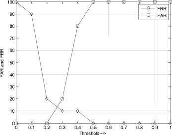
Fig.5. FAR and FRR versus Threshold on YALE Database
Table 5. Performance on Yale Database with Pre-processing Methods
|
Threshold |
SSR |
MSR |
SSQ |
||||||
|
% FRR |
% FAR |
% RR |
% FRR |
% FAR |
% RR |
% FRR |
% FAR |
% RR |
|
|
0.0 |
100 |
0 |
0 |
100 |
0 |
0 |
100 |
0 |
0 |
|
0.1 |
80 |
0 |
20 |
90 |
0 |
10 |
90 |
0 |
10 |
|
0.2 |
30 |
0 |
60 |
20 |
0 |
70 |
40 |
0 |
60 |
|
0.3 |
10 |
20 |
70 |
10 |
20 |
80 |
20 |
0 |
80 |
|
0.4 |
10 |
80 |
70 |
10 |
80 |
80 |
0 |
80 |
80 |
|
0.5 |
0 |
100 |
80 |
0 |
100 |
90 |
0 |
100 |
90 |
|
0.6 |
0 |
100 |
80 |
0 |
100 |
90 |
0 |
100 |
90 |
|
0.7 |
0 |
100 |
80 |
0 |
100 |
90 |
0 |
100 |
90 |
|
0.8 |
0 |
100 |
80 |
0 |
100 |
90 |
0 |
100 |
90 |
|
0.9 |
0 |
100 |
80 |
0 |
100 |
90 |
0 |
100 |
90 |
|
1.0 |
0 |
100 |
80 |
0 |
100 |
90 |
0 |
100 |
90 |
Table 6. EER and %RR Comparison on Yale Database
|
Method |
EER |
Optimum % RR |
Maximum %RR |
|
SSR |
14 |
68 |
80 |
|
MSR |
13 |
78 |
90 |
|
SSQ |
16 |
80 |
90 |
-
B. Performance on GTAV database
The GTAV database images of faces for thirty persons each with sixteen images per person is used for database. One image is used as the test image for FRR calculation and tenth out of database image of ten persons is used for FAR calculation. The performance of with SSR, MSR, and SSQ preprocessing methods are in Table 8. The Maximum %RR of 90, 90, and 93.33 is obtained for SSR, MSR, and SSQ preprocessing methods respectively. ED is used to compute the results on GTAV face database. The metrics such as EER, Optimum % RR, and Maximum %RR are compared in Table 9 for SSR, MSR, and SSQ preprocessing methods in the proposed work. Minimum EER of 19 is obtained for SSQ preprocessing method, but the Optimum % RR and Maximum %RR are 75 and 93.33 respectively. Figure 6 depicts the plot of FAR and FRR versus Threshold on GTAV database using SSQ preprocessing. Table 10 Compares the maximum %RR of other algorithm with the proposed work. It is justified that the Maximum %RR is higher compared to [34] on GTAV face database. ED is used to compute the results on GTAV face database.
Table 7. Maximum %RR Comparison with Other Methods on YALE Database
|
Method |
Maximum % RR |
|
ALBP +BCD [31] |
71.9 |
|
WM(2D)2PCA[32] |
80.77 |
|
GABOR +DTW [33] |
90.67 |
|
Proposed MDE-D3S FR model |
90 |
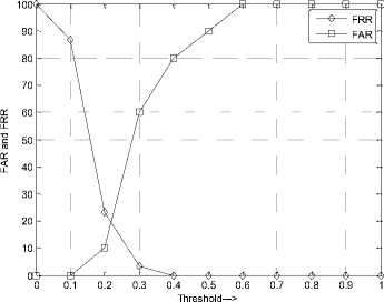
Fig.6. FAR and FRR versus Threshold on GTAV Database
Table 8. Performance on GTAV Database with Pre-processing Methods
|
Threshold |
SSR |
MSR |
SSQ |
||||||
|
% FRR |
% FAR |
% RR |
% FRR |
% FAR |
% RR |
% FRR |
% FAR |
% RR |
|
|
0.0 |
100 |
0 |
0 |
100 |
0 |
0 |
100 |
0 |
0 |
|
0.1 |
63.33 |
0 |
33.33 |
70 |
0 |
30 |
86.67 |
0 |
13.33 |
|
0.2 |
10 |
30 |
86.67 |
13.33 |
40 |
86.67 |
23.33 |
10 |
70 |
|
0.3 |
0 |
70 |
90 |
0 |
70 |
90 |
3.33 |
60 |
90 |
|
0.4 |
0 |
90 |
90 |
0 |
90 |
90 |
0 |
80 |
93.33 |
|
0.5 |
0 |
100 |
90 |
0 |
100 |
90 |
0 |
90 |
93.33 |
|
0.6 |
0 |
100 |
90 |
0 |
100 |
90 |
0 |
100 |
93.33 |
|
0.7 |
0 |
100 |
90 |
0 |
100 |
90 |
0 |
100 |
93.33 |
|
0.8 |
0 |
100 |
90 |
0 |
100 |
90 |
0 |
100 |
93.33 |
|
0.9 |
0 |
100 |
90 |
0 |
100 |
90 |
0 |
100 |
93.33 |
|
1.0 |
0 |
100 |
90 |
0 |
100 |
90 |
0 |
100 |
93.33 |
Table 9. EER and %RR Comparison on GTAV Database
|
Method |
EER |
Optimum %RR |
Maximum %RR |
|
SSR |
22 |
60 |
90 |
|
MSR |
28 |
60 |
90 |
|
SSQ |
19 |
75 |
93.33 |
Table 10. Maximum %RR Comparison with Other Method on GTAV
Database
|
Method |
Maximum % RR |
|
P2CA [34] |
78 |
|
Proposed MDE-D3S FR Model |
93.33 |
-
C. Performance on ORL database
The ORL database images of faces for twelve persons each with eight images per person is used for database. One image is used as the test image for FRR calculation and ninth out of database image of twenty eight persons is used for FAR calculation. Performance of the proposed algorithm with preprocessing methods such as SSR, MSR, and SSQ is in Table 11. The Maximum %RR attained is 100 for all the three preprocessing methods. ED is used to compute the results on ORL face database.
Performance metrics for the proposed work such as EER, Optimum % RR, and Maximum %RR are tabulated in Table 12 for SSR, MSR, and SSQ preprocessing methods. EER is minimum of 16 for SSR preprocessing method, but the Optimum % RR and Maximum %RR are 85 and 100 respectively. Table 13 Compares the Maximum %RR of other algorithms such as [32], [33], [35], [36] and [37] with proposed work, which proves by attaining the maximum value. The plot of FAR and FRR versus Threshold on ORL database using SSR preprocessing is in Figure 7.
The reasons for result improvement are; SSR, MSR, and SSQ preprocessing methods used are linear in process to reduce the nonlinear effect of image details. Irrespective of the image information contained before preprocessing, the output image is normalized using
Gaussian filters, to yield smooth image. The Approximate band of DWT has linear relationship with the input image, but neglects the edge information. EDBC extracts directional information related to high frequency details affined to edges and other variations of the image. Hence EDBC features have good discrimination power among different persons. Schur, Hessenberg and QR matrix decompositions are individually nonlinear in nature, but have less number of nonzero coefficients when all are combined. It is found by analysis that the matrix decompositions are able to discriminate different persons efficiently, but has more similarities between the images of a same person. Singular values of SVD have bounded good energy, as the ratio of input and output is 10:1.
Fusing EDBC and SVD features has good discrimination ability between two different persons and it is justified from Table 14, in terms of AOD. Minimum AOD value of 34.15 is observed between two images of same person on Yale database, and maximum AOD value of 95.88 is reported for the images of two different persons of ORL database.
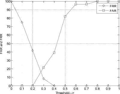
Fig.7. FAR and FRR versus Threshold on ORL Database
Table 11. Performance on ORL Database with Pre-processing Methods
|
Threshold |
SSR |
MSR |
SSQ |
||||||
|
% FRR |
% FAR |
% RR |
% FRR |
% FAR |
% RR |
% FRR |
% FAR |
% RR |
|
|
0.0 |
100 |
0 |
0 |
100 |
0 |
0 |
100 |
0 |
0 |
|
0.1 |
75 |
0 |
25 |
100 |
0 |
0 |
83.33 |
0 |
16.67 |
|
0.2 |
41.67 |
0 |
58 |
83.33 |
0 |
16.67 |
41.67 |
0 |
58.33 |
|
0.3 |
8.33 |
21.42 |
91.67 |
50 |
0 |
50 |
16.67 |
17.85 |
83.33 |
|
0.4 |
0 |
39.28 |
100 |
25 |
7.14 |
75 |
0 |
42.85 |
100 |
|
0.5 |
0 |
82.14 |
100 |
8.33 |
39.28 |
91.67 |
0 |
82.14 |
100 |
|
0.6 |
0 |
96.42 |
100 |
0 |
82.14 |
100 |
0 |
96.42 |
100 |
|
0.7 |
0 |
96.42 |
100 |
0 |
100 |
100 |
0 |
96.42 |
100 |
|
0.8 |
0 |
100 |
100 |
0 |
100 |
100 |
0 |
100 |
100 |
|
0.9 |
0 |
100 |
100 |
0 |
100 |
100 |
0 |
100 |
100 |
|
1.0 |
0 |
100 |
100 |
0 |
100 |
100 |
0 |
100 |
100 |
Table 12. EER and % RR Comparison on ORL Database
|
Method |
EER |
Optimum % RR |
Maximum %RR |
|
SSR |
16 |
85 |
100 |
|
MSR |
17 |
83.33 |
100 |
|
SSQ |
19 |
85 |
100 |
Table 13. Maximum % RR comparison with Other Methods on ORL Database
|
Method |
Maximum % RR |
|
WM(2D)2PCA [32] |
74.06 |
|
GABOR +DTW [33] |
86.38 |
|
Gabor + SVM RFE [35] |
93.5 |
|
OOLPP2+SVM2 [36] |
94 |
|
BTSS [37] |
99.5 |
|
Proposed MDE-D3S FR model |
100 |
Table 14. AOD Comparison of Fused Features on Three Databases
|
Database |
Between Two images of Person1 |
Between Two images of Person2 |
Between Person2 and Person1 |
|
YALE |
53.36 |
34.15 |
61.59 |
|
GTAV |
40.39 |
47.91 |
70.91 |
|
ORL |
63.5 |
66.5 |
95.88 |
-
VI. Conclusion
Person recognition using faces have no unique solutions in multidimensional constraints environment. The MDE-D3S FR model proposed in this work, utilizes three preprocessing methods such as SSR, MSR, and SSQ. DWT is applied on preprocessed image of size 100*100. On the LL band of DWT, EDBC is applied to extract one hundred features. In other part of the algorithm, preprocessed image is decomposed using Schur, Hessenberg and QR methods and SVD is applied on the sum of three decompositions to get another one hundred features. EDBC and SVD features are linearly added to yield final one hundred features. The matching results using City-block or Euclidean Distance (ED) measures are computed. The performance on three publically available databases such as YALE, GTAV and ORL are superior compared with other existing methods.
References Synergy of Schur, Hessenberg and QR Decompositions on Face Recognition
- Alexander Andreopoulos and John K. Tsotsos, "50 Years of object recognition: Directions Forward," ELSEVIER International Journal on Computer Vision and Image Understanding, Vol. 117, Issue. 7, pp. 827-891, August 2013.
- Giovanni Betta, Domenico Capriglione, Mariella Corvino, Consolatina Liguori, and Alfredo Paolillo, "Face Based Recognition Algorithms: A First Step Toward a Metrological Characterization," IEEE Transactions on Instrumentation and Measurement, Vol. 62, No. 5, pp. 1008 – 1016, May 2013.
- Yuanzheng Li, "Smile Recognition Based on Face Texture and Mouth Shape Features," IEEE Workshop on Electronics, Computer and Applications, pp. 606 – 609, May 2014.
- Hamdi Dibeklioğlu, Albert Ali Salah, and Theo Gevers, "Recognition of Genuine Smiles" IEEE Transactions on Multimedia, Vol. 17, No. 3, pp. 279 – 294, March 2015.
- Senthil Singh and Manikandan, "Face Recognition using Relationship Learning Based Super Resolution Algorithm," American Journal of Applied Sciences, Vol. 11, Issue 3, pp. 475-481, January 2014.
- Hu Han, ShiguangShan, XilinChen, and WenGao, "A Comparative Study on Illumination Preprocessing in Face Recognition," ELSEVIER International Journal on Computer Pattern Recognition, Vol. 46, Issue 6, pp. 1691–1699, June 2013.
- Gopinath Mahale, Hamsika Mahale, Arnav Goel, S.K.Nandy, S.Bhattacharya,and Ranjani Narayan, "Hardware Solution For Real-time Face Recognition," Twenty Eighth IEEE International Conference on VLSI Design and Embedded Systems, pp. 81 – 86, January 2015.
- Jianling Hu, Lei Shao, and Honglong Cao, "Design and Implementation of an Embedded Face Recognition System on DM642," Springer-Verlag Berlin Heidelberg – Advances on Digital Television and Wireless Multimedia Communications, Communications in Computer and Information Science, Vol. 331, pp. 448–458, November 2012.
- Meng Joo Er, Weilong Chen, and Shiqian Wu, "High-Speed Face Recognition Based on Discrete Cosine Transform and RBF Neural Networks," IEEE Transactions on Neural Networks, Vol. 16, No. 3, pp. 679 – 691, May 2005.
- Gorti Satyanarayana Murty, J SasiKiran, and V Vijaya Kumar, "Facial Expression Recognition based on Features Derived from the Distinct LBP and GLCM," International Journal of Image, Graphics and Signal Processing, Vol. 6 , No. 2, pp. 68-77, January 2014.
- Linlin Shen and Jinwen He, "Face Recognition with Directional Local Binary Patterns," Springer-Verlag Berlin Heidelberg – Sixth Chinese Conference on Biometric Recognition, Lecture Notes in Computer Science, Vol. 7098, pp. 10–16, December 2011.
- Zheng-Hai Huang, Wen-Juan Li, Jun Wang, and Ting Zhang, "Face Recognition based on Pixel Level and Feature Level Fusion of the Top Level's Wavelet Sub Bands," ELSEVIER International Journal on Information Fusion, Vol. 22, pp. 95–104, March 2015.
- Shahan Nercessian, Karen Panetta and Sos Agaian" Image Fusion Using the Parameterized Logarithmic Dual Tree Complex Wavelet Transform," IEEE International Conference on Technologies for Homeland Security, pp. 296 -302, November 2010.
- Aruni Singh, and Sanjay Kumar Singh, "Effect of Face Tampering on Face Recognition," An International Journal on Signal & Image Processing, Vol.4, No.4, pp. 83 – 99, August 2013.
- Chung-Hao Chen, Yi Yao, Hong Chang, Andreas Koschan, and Mongi Abidi, "Integration of Multispectral Face Recognition and Multi-PTZ Camera Automated Surveillance for Security Applications," VERSITA -Central European Journal on Engineering, Vol. 3, Issue 2, pp. 253-266, June 2013.
- Jagadeesh H S, Suresh Babu K, and K B Raja, "Face Recognition based on Spatial and Transform Domain Techniques," International Journal of Computer Science and Information Security, Vol.13, No. 09, pp. 6- 14, September 2015.
- http://vision.ucsd.edu/datasets/yale_face_dataset_original/yalefaces.zip.
- http://gps-tsc.upc.es/GTAV/ResearchAreas/ UPCFaceDatabase/ GTAVFaceDatabase.htm.
- F Samaria and A Harter, "Parameterization of a stochastic model for human face identification," Second IEEE Workshop on Applications of Computer Vision, pp. 95–104, December 1994.
- Struc and N Pavesic, "Performance Evaluation of Photometric Normalization Techniques for Illumination Invariant Face Recognition", In: Y.J. Zhang (Ed.), Advances in Face Image Analysis: Techniques and Technologies, IGI Global, 2010.
- Struc and N Pavesic, 2009, "Gabor based Kernel Partial Least Squares Discrimination Features for Face Recognition," Informatica (Vilnius), Vol. 20, No. 1, pp. 115–138, 2009.
- D J Jobson, Z Rahman, and G A Woodell, "Properties and Performance of a Center / Surround Retinex," IEEE Transactions on Image Processing, Vol. 6, No. 3, pp. 451–462, March 1997.
- E H Land, and J J McCann, "Lightness and Retinex Theory," Journal of the Optical Society of America, Vol. 61, Issue 1, pp. 1–11, January 1971.
- D J Jobson, Z Rahman, and G A Woodell. "A Multiscale Retinex for Bridging the Gap between Color Images and the Human Observations of Scenes," IEEE Transactions on Image Processing, Vol. 6, No. 7, pp. 965–976, July 1997.
- H Wang, S Z Li, Y Wang, and J Zhang, "Self Quotient Image for Face Recognition," IEEE Proceedings of the International Conference on Pattern Recognition, pp. 1397- 1400, October 2004.
- Hafiz Imtiaz and Shaikh Anowarul Fattah, "A Wavelet-domain Local Feature Selection Scheme for Face Recognition," IEEE Symposium on Computers and Informatics, pp. 448 - 451, March 2011.
- Gheorghita Ghinea, Rajkumar Kannan, and Suresh Kannaiyan, "Gradient-Orientation-Based PCA Subspace for Novel Face Recognition," IEEE OPEN ACCESS Journal, Vol. 2, pp. 914 – 920, August 2014.
- Yulu Jia, George Bosilca, Piotr Luszczek and Jack J. Dongarra, "Parallel Reduction to Hessenberg Form with Algorithm-Based Fault Tolerance," ACM Proceedings of the International Conference on High Performance Computing, Networking, Storage and Analysis, Article No. 88, pp.1 – 11, November, 2013.
- Sheng Zhang and Terence Sim, "When Fisher Meets Fukunaga-Koontz: A New Look at Linear Discriminants," IEEE Proceedings of the Computer Society Conference on Computer Vision and Pattern Recognition, Vol. 1, pp. 323 - 329, June, 2006.
- Ashish M Kothari, and Ved Vyas Dwivedi, "Hybridization of DCT and SVD in the Implementation and Performance Analysis of Video Watermarking," International Journal of Image, Graphics and Signal Processing, Vol. 4, No. 5, pp. 14-20, June 2012.
- Radhey Shyam and Yogendra Narain Singh, "Face Recognition using Augmented Local Binary Pattern and Bray Curtis Dissimilarity Metric," Second IEEE International Conference on Signal Processing and Integrated Networks, pp. 779 – 784, February, 2015.
- Erhu Zhang, Yongchao Li, and Faming Zhang, "A Single Training Sample Face Recognition Algorithm Based on Sample Extension," Sixth IEEE International Conference on Advanced Computational Intelligence, pp. 324- 327, October, 2013.
- Venkatramaphanikumar S and V Kamakshi Prasad, "Gabor Based Face Recognition with Dynamic Time Warping," Sixth IEEE International Conference on Contemporary Computing, pp. 349 - 353, August, 2013.
- Antonio Rama and Francesc Tarrés, "Face Recognition using a Fast Model Synthesis from a Profile and a Frontal View," IEEE International Conference on Image Processing, Vol. 4, pp. 501- 504, October, 2007.
- Xianqiang Lv, Junfeng Wu, and Wei Liu, "Face Image Feature Selection based on Gabor Feature and Recursive Feature Elimination," Sixth IEEE International Conference on Intelligent Human-Machine Systems and Cybernetics, Vol. 2, pp. 266 – 269, August 2014.
- John Soldera, Carlos Alberto Ramirez Behaine, and Jacob Scharcanski, "Customized Orthogonal Locality Preserving Projections With Soft-Margin Maximization for Face Recognition," IEEE Transactions on Instrumentation and Measurement, Vol. 64, No. 9, pp. 2417 - 2426, September 2015.
- Yong Xu, Xiaozhao Fang, Xuelong Li, Jiang Yang, Jane You, Hong Liu, and Shaohua Teng, "Data Uncertainty in Face Recognition," IEEE Transactions on Cybernetics - Biometrics Compendium, Vol. 44, Issue, 10, pp. 1950 – 1961, January, 2014.
