Technical system simulation with Python

As part of the implementation of the project "Space mission ReshUCube-3", the laboratory of small spacecraft (SSC) of Reshetnev University together with the laboratory of Space systems and technologies of the FRC KSC SB RAS is developing an orientation system for a small satellite of the CubeSat 1U format. It has an active magnetic orientation system, the structure of which is shown in Fig. 1. It is a classical system with feedback.

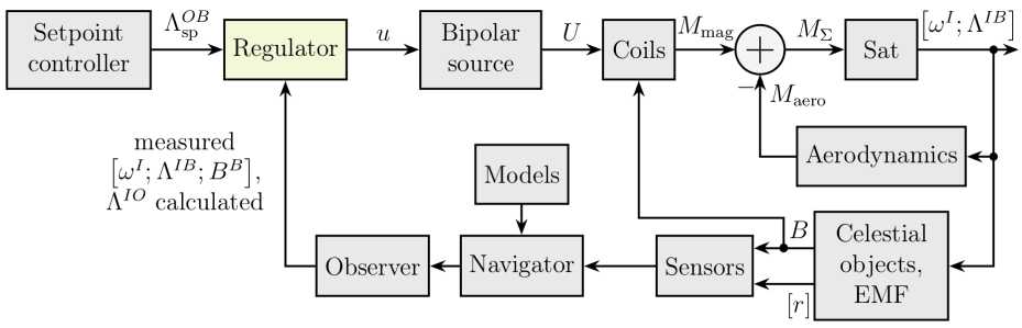
Рис. 1. Структурная схема системы ориентации КА ReshUCube-3

Fig. 1. ADCS of ReshUCube-3 structure

The state of the spacecraft (SC) is described by the angular velocity ω ^I and the rotation quaternion Λ ^IB of the associated coordinate system (superscript B, body axes) relative to the inertial space (I, inertial). The state depends on the applied rotational moment, which is composed of the moment from the M aero aerodynamic forces and the magnetic moment M magn . The controlling moment is the magnetic moment, which is created by the interaction of the magnetic fields of the electromagnetic device (EMD, magnetic coil) and the vector B of the Earth's magnetic field (EMF).

Several coordinate systems are used to control the orientation - some vectors are simply more convenient to specify in their own coordinate system. Firstly, this is a bound coordinate system (body axes, index B), the axes of which are rigidly connected to the apparatus and rotate together with it. They are usually located along the construction axes of the spacecraft. Secondly, the inertial coordinate system (inertial, index I), which is tied to the inertial space, to the direction to the stars. It does not rotate. Thirdly, the orbital coordinate system (orbital, index O), always directed by the x O axis to the center of the Earth (along the local vertical), and the x O axis is directed along the spacecraft velocity vector. This system is convenient for determining the direction to the Earth and taking into account aerodynamic forces and moments. The superscripts of a vector or quaternion indicate in which of the coordinate systems its components are taken.

The control device generates a control signal in such a way that the measured rotation quaternion Λ ^IB meas becomes equal to the desired quaternion Λ ^IB des , i.e., so that the spacecraft takes the specified orientation. In form, this is a classic PD controller for such tasks (for the D-channel, the angular velocity ω ^I meas is used). An excellent review of the current state of magnetic orientation systems is given in [1].

In the given control system, the navigation algorithm and the observer algorithm are quite complex, which, based on sensor readings, calculate the most statistically reliable values of the spacecraft state variables.

In the structural diagram, it is possible to distinguish groups of blocks that have different natures. For example, spacecraft rotations, aerodynamic and magnetic moments have a physical nature and act continuously; the controller, observer and navigator are algorithms that operate in the onboard computer with some periodicity. It is clear that in simulation modeling, these groups must be calculated using different computational methods, linking them into a single calculation in order to obtain a joint solution.

This calculation method is called co-simulation, the essence of which is as follows. Simulation models of parts of the system are combined with their calculation method (solver) into calculation modules. The modules are sequentially, in the order specified by the system structure, launched for calculation at a certain step of model time. The calculation results are transmitted as initial conditions for the modules following in the calculation order. Thus, the modules are interconnected, and the overall solution is joint.

Problem Status Overview

A good and very detailed overview of the current state of this technology is given in [2]. Intermodular interaction is provided by an orchestrator - a module manager that sets the model time, determines the order of launching modules for calculation and ensures the transfer of data between modules, from the output to the inputs of the next one.

ALGORITHM 3: Generic Jacobi-based orchestrator for autonomous CT co-simulation scenarios.

Data: An autonomous scenario cs = (0, Y_CS,D = (1,... ,n}, {Si} ,L,0), and a communication step size H.

Result: A co-simulation trace.

t := 0;

Xi := Xi (0) for i = 1,n; while true do

Solve the following system for the unknowns:

(J/l = ^(t^^Ui)

Уп — ^n (L x_n, u_n)

ШУь • .^Уп^Щ,---,^) = 6

X{ := 8i(t,Xi,Ui), for i = 1,... ,n;                            // Instruct each SU to advance t := t + H;                                                           // Advance time end

Рис. 2. Алгоритм оркестратора для систем с непрерывным временем [2]

Fig. 2. Orchestrator algorithm for continuous-time stystens [2]

Fig. 2 shows a generalized orchestrator algorithm for continuous-time systems. It explicitly identifies a cycle over model time, in which:

• 1.    Model outputs are calculated taking into account the imposed constraints. Here, a system of nonlinear equations is solved that calculates the operating point of the system.

• 2.    Model state variables for the next step are calculated.

• 3.    Step H is taken over time.

The cycle is performed until the final time is reached.

In the given algorithm, λ(t, x, u) is the function for calculating the model output y; x and u are the state variables and inputs of the model; δ is the function for calculating the system state variables; H is the time step size; L is the functional that specifies the constraints.

The authors of [2] distinguish discrete, continuous and hybrid models depending on the type of interaction of models in time. They differ in the features of orchestration during joint calculation. The review considers in detail the problems of joint modeling specific to each type of system, for example, the use of constraints imposed on solutions, algebraic cycles, strategies for initializing models at the operating point, control of convergence and stability of the solution, accuracy and validity of coupled models.

In practice, inter-model interaction is implemented in different ways. A common pattern is the "Publisher-Subscriber" message transfer pattern [3], in which a message (e.g., a calculation result) is placed by the publisher in a data transfer channel or database, and the subscriber selects only the messages it specifically requires.

In some implementations, the publisher sends messages to an intermediary (broker). In this case, subscribers must register a subscription with the broker, which stores and forwards messages to the subscriber. Subscribers can subscribe to specific messages at the coding stage, during application initialization, or during execution.

For example, the well-documented HELICS (Hierarchical Engine for Large-scale Infrastructure CoSimulation) framework [4] uses a broker that organizes inter-model communications (provides information about model interfaces), and message exchange occurs at the horizontal model-to-model level, bypassing the broker (Fig. 3). Subscription uses JSON configuration files that are read during initialization. In addition, in HELICS, the broker functions as an orchestrator, synchronizing message exchange.

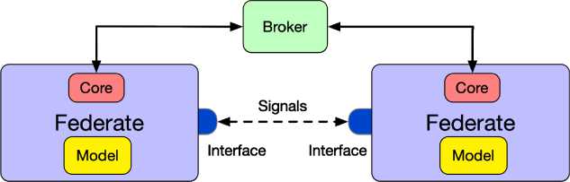
Рис. 3. Базовая архитектура фреймворка HELICS [5]. Здесь Federate – вычислительный модуль с ядром Core (управление моделированием и интерфейс сообщений) и выполняемым кодом модели

Fig. 3. Base architecture of HELICS framework [5]. Here Federate is a computational module containing a core (simulation control and message interface) and executable model code

The architecture of the MOSAIC package, written entirely in Python, includes a core and a set of interfaces (Fig. 4). The core, in which the orchestrator is implemented, consists of two components: a scheduler and a model coordinator.

The user writes a script that sets the modeling mode. Based on the script, the scheduler determines the parameters of the models, ensures the sequence of execution and synchronization of the models, and acts as a broker for data exchange. The coordinator is responsible for communication between models, using interfaces for specific protocols for inter-model data exchange.

In the domestic simulation modeling complex SimInTech, a broker is not used: the model does not register signals, but simply takes them by requests to the common intermodel signal database. The architecture of the complex is shown in Fig. 5.

The SimInTech complex is a system with model compilation into machine code, which allows for very fast simulation. To set up custom control algorithms containing complex operations for processing sensor signals and calculating control, a built-in programming language is used. It is a dialect of the Pascal language adapted for the tasks of programming simulation models operating in time. For example, it includes code sections that are executed at individual stages of simulation (compilation, initialization, finalization), there are capabilities for accessing system functions and variables, as well as for working with a model signal database, etc.

The language is quite deeply specialized and is not fully compatible with the Pascal language (for example, there is no way to set complex types of variables and objects), there are no third-party compilers and debuggers for it.

The latest versions of SimInTech have integration with the Python programming language - you can execute a script once (for example, during initialization). Since Python code is not compiled, it will take quite a long time to execute when executed cyclically (starting the interpreter, passing the script and parameters, execution, passing the results).

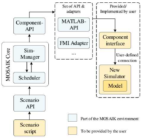
Рис. 4. Архитектура фреймворка MOSAIC [6]

Fig. 4. Architecture of MOSAIC framework [6]

It is executed by a Python interpreter external to SimInTech, and with this method of launching it is extremely difficult to implement storage of the state of objects (this was required for the SGP4 algorithm, which determines the current position of the spacecraft [7]).

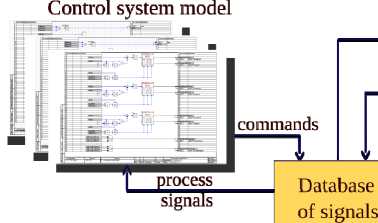
control signals process variables

Electrical model

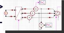
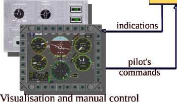
Рис. 5. Архитектура комплекса имитационного моделирования SimInTech [8]

Fig. 5. Architecture of SimInTech dynamic simulation environment [8]

Mechanical model

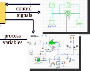
Thermohydraulical model

SimInTech allows you to develop a block with your own algorithms using external SimInTech tools (for example, in the form of a dynamic .dll library), but the creation procedure is described only for Windows, using the Delphi environment. In 2020, the SimInTech system was successfully ported to Linux OS [9], but, unfortunately, to date there is no description of the procedure for creating and connecting blocks in the form of dynamic .so libraries. Debugging in the SimInTech programming environment is not very convenient, although all the basic tools are available (breakpoints, viewing the state of variables, etc.). The static code analyzer (linter) is not implemented. As a result, a number of features of the software discussed above did not allow the implementation of the orientation system model in it; the code was quite cumbersome, fast-growing and difficult to debug.

Therefore, it was decided to rewrite all algorithms and models in Python, for the joint execution of which a dispatcher was written for the joint execution of models calculated by different algorithms.

Considering modeling systems implemented using Python, we should mention the excellent and well-developed Basilisk system [10], developed at the Astrodynamics Research Center of the University of Colorado. This compiled system is written in C++, and the Python code is linked (and compiled) to the system via the Software Interface Generator (SWIG). Accordingly, the models are executed quite quickly. Basilisk was written specifically for modeling space systems and has a very good graphics subsystem. It also has the ability to connect C++ code, implement hardware-in-the-loop technologies, as well as software-in-the-loop programs. Like all programs with extensive functionality, well-developed and with a long history, Basilisk is quite difficult to use, but this complexity is fully justified. Frankly speaking, if at the time when the author started working on the orientation system, the Basilisk system had been encountered, then it is unlikely that the development of his own modeling system would have begun.

The orientation system model presented in the report [11] is written entirely in Python. Its peculiarity is that it uses a simplified technology of joint modeling: a common matrix of equations is formed, solved by the LSODA algorithm for continuous systems per time step; then the orientation system algorithms are executed. The system has algorithms and equations of individual blocks, each of which ensures the formation of its part of the equation system.

Architecture

Figure 6 shows the architecture of a dispatcher for simulation modeling of control systems.

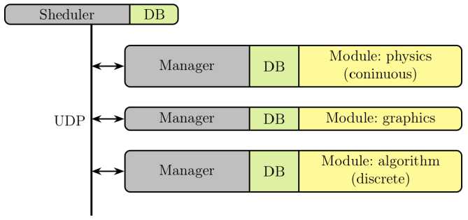
Рис. 6. Архитектура диспетчера имитационного моделирования pySimScheduler [12]

Fig. 6. Architecture of dynamic simulation model manager pySimScheduler [12]

Each model is implemented as an independent calculation module. It is launched in a separate process and contains both the equations and algorithms of the model, and the methods of numerical calculation of these algorithms. The module must calculate its output values for a certain time interval.

Similar to how it is implemented in SimInTech, the module can be in several states (Fig. 7). The transition between these states occurs according to the dispatcher commands or in response to the module's internal events.

After receiving the command to start the simulation, the module switches (A) from the Idle waiting state to the Run working state; in this case, the graphics and internal variables of the module are initialized (the initial state is set). After this, the dispatcher cyclically issues a command to each calculation module to perform a calculation step (B), passing the initial data (the calculation result of the modules adjacent to it) to the module and taking the calculation results (to pass them on to subsequent modules). At the end of the calculation time, the module switches to the waiting state (C), performing actions to finalize the calculation (finishing the graphics, closing files). If an internal error occurs during the calculation, the module switches to the error state (E) with the error message to the dispatcher,

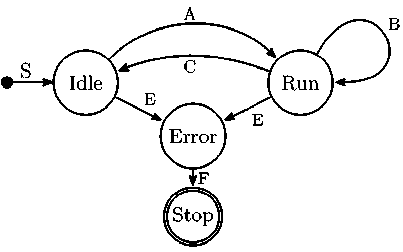
Рис. 7. Машина состояний системы pySimScheduler

Fig. 7. State machine of pySimScheduler model manager

and then stops. In this case, on the command of the dispatcher, the remaining modules switch to the waiting state.

Data exchange is performed via UDP packets, which contain variables from the common database required for a specific module. Each module contains a database manager. It unpacks/packs packets and distributes data according to the internal variables of the module class. The system is based on [13], where exchange is performed with the equipment of the stand, which works like a calculation module.

The database must contain the actual database of variables that will be common between modules. It also contains a list of modules indicating which vari- ables participate in the exchange (which are transmitted, and which are received).

After the module is initialized, a Manager object will appear in its attributes, which is the database manager. It will create (during its initialization) the required attributes in the module object, which are fields of the common database – they will be synchronized at each calculation step.

The general database, its fields, and the composition of specific variables for exchange with specific modules are set in the container class in the form of attributes:

Listing 1. Sample database code class DataBase():

• #    --- common variables ---

• t    = 0. # model time

dt = 0.25 # calculation step tmax = 4. # simulation time cmd = 0 # command to all modules

• #    --- user variables ---

• U = np.array([0.1, 0., 0.]) # control

Modules are called in the order they appear in the Tasks dictionary. For example, Listing 2 specifies three modules (Rotation, Control, and Plot2D), whose names are keys in this dictionary:

Listing 2. Example of defining module call parameters

Tasks = {

'Rotation':{'Keys':"""t,cmd,dt,

U,L_B,B_I,Mm_B, w_B, q_IB"""},

'Control':{'Keys':['t','cmd','U','B_I','q _IB']},

'Plot2D': {'Keys':'t,cmd,dt,U,w_B,q_IB',

'Addr':('188.162.92.100', 6502),

'noAnswer':True}

The values corresponding to the keys are also dictionaries (dict). They have a mandatory Keys, which specifies the database fields that will be exchanged with this module at the specified address.

If data is exchanged with a remote system, then it is necessary to specify the network address to which data packets will be sent. In this case, the Addr key is added, the value of which must be a tuple and have the form (ip address, port).

It is possible to configure the exchange so that the module does not return data, but only receives them. This is convenient when the module solves computationally difficult problems of visualizing twodimensional and three-dimensional graphs. In order not to wait for an answer, the noAnswer flag is used.

Since standard methods for solving differential and other equations are used to obtain a joint solution in each of the models, and data exchange is completely predictable, the joint solution will be adequate and accurate. It is clear that for a stable solution, the question of choosing the step length of variable exchange arises. It is considered in many publications (see review [2]), and with a reasonable approach to choosing the parameters of the solution methods, the joint solution will be adequate.

Writing and executing models

The model code looks like a description of a Python class, which must have methods with specific names that are called during transitions between states. It is necessary to specify the calculation code of the model in them. The state machine (see Fig. 7) and the database manager are implemented in the parent class, from which the class with the model description must be inherited.

From the code, it is clear that it is necessary to override (if necessary) the following methods, specifying the required model logic in them:

• –    Setup – is run once when an instance of the model class is created;

• –    Initialize – is executed once during model initialization before running the calculation;

• –    Run – model calculation. It is cyclically for each time interval dt;

• –    Finalize – is executed once, at the end of the calculation.

On transitions to the Error and Stop states, the module's internal service methods are executed, into which the user should not enter the model logic.

At the end of the file with the model code, you need to create an instance of the class and transfer control to the internal state machine:

The parameters of the model class are specified:

• –    TaskList: list of modules Tasks;

• –    DB: shared database object;

• –    isSheduler: a flag indicating whether the module contains a dispatcher and runs other modules. One of the modules must be the master module, run all the others and ensure data exchange. It must have the isSheduler=True flag and be run last. It is convenient to make the module whose code we are currently working with the master module;

• –    isRealTime: flag indicating whether we are working in real time (the t attribute corresponds to real time). This mode is usually used when exchanging data with real equipment.

Each module must be run in a separate Python interpreter, with the console displaying the module's state. After the master module has been launched, the system begins to simulate - it runs the state machine. After the simulation time has expired, the slave modules go into the Idle state and wait for further commands. When restarting, the model uses the initial conditions specified in the database at the time of Setup; initial conditions can be specified directly in the model code.

Application

To determine the quaternion of the spacecraft rotation relative to the inertial space, the navigator algorithm is used.

Let a set of unit “measured” vectors b be received from the sensors in the current angular and spatial position of the spacecraft, presented in a related coordinate system. For a small spacecraft with a limited set of sensors, this could be, for example, the direction to the Sun, Earth, and the EMF vector.

Also, for the current spatial position of the spacecraft, the same vectors are calculated – a set of “standard” (reference) unit vectors r . They are specified in the inertial reference system.

It is necessary to find a rotation that will combine the reference vectors with the measured vectors with the smallest error. This rotation will determine the angular position of the associated coordinate system relative to the inertial one.

The calculation of reference vectors must be performed on board. The initial data for this algorithm are the spacecraft coordinates in the inertial coordinate system, which are calculated based on the TLE parameters using the SGP4 algorithm. This is a fairly complex algorithm (Fig. 8), proposed in [14] and translated into many programming languages. To determine the coordinates, the TLE parameters are transmitted to the spacecraft from time to time (at intervals of approximately one week). The SGP4 algorithm is quite resource-intensive, and therefore the exact calculation is performed periodically (daily), and between its calls an approximate, extrapolated solution is calculated.

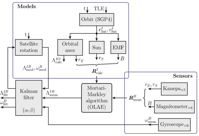
Рис. 8. Структура алгоритма навигатора

Fig. 8. Navigation algorithm structure

In the simulation model of the system, calculation of reference vectors is also required for sensor models. In this case, the algorithm models the surrounding world – the “real” position of the Sun and the vector of the EMF, calculating the corresponding vectors r * in the inertial system. Based on these vectors, the sensor model forms the measured vectors b , adding noise and bias.

If the vectors r and r * are calculated using the same algorithm, they will differ only in the added noise. Therefore, to increase the robustness of the system, it was decided to use different implementations of the algorithms: in the onboard software, to use the C/C++ code from [7; 15], and in the sensor model, to use the OreKIT astrodynamics library [14].

A simplified manager was developed to link the C++ code with the dispatcher, which is written in Python. It implements a similar state machine (see Fig. 5), calling the necessary procedures for initialization (required for the SGP4 algorithm), calculation per time step, and finalization of the model. Since the format of structures in Python and C++ is different, the cppystruct library [17] is used to work with UDP packets on the model side. It allows unpacking and packing UDP packets into a format accepted by the struct library (an example of the code is given in the ex5.1 directory of the repository [13]). At the moment, the manager code is formed by calling a special dispatcher method; the code will form a C++ structure with field names corresponding to variables in the database. The programmer must independently set calls to the necessary procedures, passing them data from this structure and filling its fields after the calculation.

Control of the spacecraft's rotational motion

Figure 9 shows the structural diagram of the rotational motion model. It details the EMU, KA and Aerodynamics blocks shown in Fig. 1.

Control with aerodynamic feedback is quite complex. A detailed examination of the control principle in this case requires a separate article. Briefly, it can be noted in advance that the aerodynamic moments have a value of about 10 % of the moments created by the magnetic orientation system. Therefore, in the first approximation, we will not take this feedback into account.

The rotational motion of a rigid body is described by two equations – dynamics and kinematics [16]. The first, the Euler equation, written in a bound coordinate system (CS) in matrix form, has the form

J doB + Ю B x (J ю B ) = MB, expressing from which the derivative of the angular velocity, we have

юB = J^1 (MB -юB x (JюB)), where J is moment of inertia tensor; ωB – angular velocity vector; MB is torque moment.

The equation of rotational kinematics, written in quaternion form, has the form

IB ¹ IB B

Л =—Л ою , where ΛIB is quaternion of rotation of the associated SC relative to the inertial space.

The moment acting on the spacecraft consists of aerodynamic and magnetic moments. The magnetic moment is used to control the motion. It is created by the interaction of the field of the coils L and the Earth's magnetic field B . Like the needle of a magnetic compass, the system of coils rotates until the vector L coincides with the Earth's field B . The rotational moment can be calculated as M = L × B .

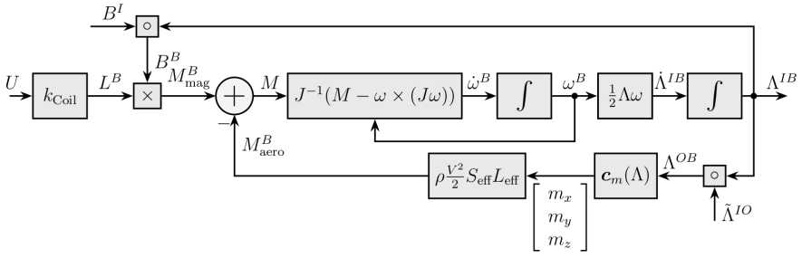
Рис. 9. Модель вращательного движения КА

• Fig. 9. Model of satellite rotational movement

For simplicity, we assume that the main feedback (including the navigation and observer algorithms) works perfectly, its coefficient is equal to one. Therefore, we close our system and consider the simplest algorithm, which is used on all (with very rare exceptions) low-flying small spacecraft - the B-Dot angular velocity damping algorithm. It is used at the initial stage of the mission to dampen the rotation that inevitably occurs after the small spacecraft is pushed out of the launch vehicle's release container.

The classic B-dot algorithm is [21]

In code, the B-dot algorithm looks simple:

Listing 4. A variant of the B-dot algorithm implementation kBDot = 500

def BDot(self):

""" B-Dot algorithm on normalized vector of Earth’s magnetic field """

Here, the Buf object is a buffer that stores the values of the variables t and B from previous iterations. They are updated in the main algorithm (see examples in the project's GitFlic repository [19]).

Fig. 10 shows the transient process for the angular velocity of the spacecraft – the component of the angular velocity ω ^B and the vector of the measured magnetic field B^B , in the axes of the associated coordinate system. It is clear how the system cannot damp the component ωX – it coincided in direction with the vector, and the magnetic system physically cannot create a moment around the vector of the magnetic field.

During rotation, the most energy-consuming axis of the spacecraft is the one with the largest moment of inertia. When the algorithm is running, when a counteracting moment is created, this component is the most difficult to extinguish. Therefore, the spacecraft almost always turns so that this axis becomes collinear to the magnetic field vector B , which is observed in the graphs of the transition process for the components of the angular velocity.

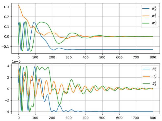
Рис. 10. Переходной процесс при гашении угловой скорости алгоритмом B-Dot

Fig. 10. Transient of B-Dot detumbling algorithm

Conclusion

The paper presents the results of developing a dispatcher designed for joint execution of simulation models that make up a multicomponent system. As a result of modeling, a joint solution to the tran sient process is obtained, which allows for complex testing of algorithms and models. This helps to identify errors that may be difficult to detect during isolated testing of individual subsystems.

A feature of the developed software is its implementation in the popular Python programming language, which allows for seamless integration of a huge number of libraries for Python, including for the development of control systems and data analysis.

Data exchange between models is performed via UDP packets, which allows using not only Python, but also other programming languages for writing models. For the same reason, it is quite simple to implement the hardware-in-loop technology (a corresponding example is given in the article [11]), which allows for more efficient development of control systems.

An example of using the developed manager to create a model of the orientation system of a small CubeSAT spacecraft with a magnetic orientation system is presented; an example of implementing the B-Dot algorithm and the results of modeling the transient process are given.

The developed system is used for simulation modeling and development of the orientation system of the ReshUCube-3 Space Mission project.

Links to the source code of the system (BSD License) are provided, which is posted in the public domain on GitFlic [21], the documentation is posted on the ReadTheDocs platform [10].